Web Interface Tutorials

Tutorial 1: Navigating the Landing Page

The Landing Page provides a single access point to all other pages in the Scout web interface and to additional information and resources on Scout.

Upon first visiting the Landing Page, you’ll see a brief summary of what Scout does and an option to “Read More” . Clicking the “Read More” button directs you to the Welcome Page of this documentation.

Scrolling down further, you’ll see brief descriptions of each of the three other pages in the Scout web interface: ECM Summaries, Analysis Results, and Baseline Energy Calculator. Clicking the “View …” links underneath each description will direct you to the page being described.

At the bottom of the landing page, a section titled “Do more with Scout” points you to resources for running your own Scout analysis from start to finish (”Quick Start Guide” button), contributing to Scout’s development on GitHub (”Contribute” button), and reporting any issues or questions you may have ( “Report an Issue” button).

The latest version of the Scout source code is accessed by clicking the “Source Code” button at the top right of the Landing Page and all other pages in the web interface.

Tip

We recommend registering an e-mail address and creating an account so that you can save your ECMs and custom analyses. To create an account, click the “Register” button on the landing page and complete the require fields.

Note

To change your username of password, after you are signed in, hover over your username and click “Profile”. On this page you will be able to change your username and/or password.

Tutorial 2: Creating and editing ECMs

The ECM Summaries Page allows you to create your own Scout ECM definitions; browse, filter and edit an existing set of ECM definitions; and upload your own set of ECMs.

Creating a new ECM or ECM package

On the ECM Summaries page, click the “Add ECM” dropdown towards the top of the page, and subsequently click “Write New ECM”. A web form will pop up that guides you step-by-step through the process of creating a new single ECM or ECM package definition. If you wish to create a single ECM definition, ensure that “Single ECM” is toggled at the top right of the form; if you wish to create an ECM package, toggle the “ECM Package” option at the top right of the form.

All inputs to the Add New ECM form are required unless they are tagged “optional”. Refer to red error messages below missing input(s) to ensure that your entries are complete.

Single ECM creation

The Add New ECM form guides you through seven steps for creating a single ECM definition, outlined below. Steps are navigated by either clicking the arrows at bottom left of the form or by clicking through the navigation bar on the left side of the form.

1. Enter general information about the ECM. Inputs include ECM name, a short description of the ECM, and an indication of whether the ECM is of the “Service Replacement” or “Add-On” type.

Note

A “Service Replacement” ECM fully replaces the service of a comparable “business-as-usual” technology (e.g., an efficient air source heat pump that replaces an existing gas furnace); an “Add-On” ECM enhances the service of the “business-as-usual” technology (e.g., a controls technology that improves the operational efficiency of an HVAC system). See Add-on type ECMs for additional guidance on this input.

Tip

Drag-and-drop an existing ECM JSON definition onto the gray box towards the bottom of the window to populate all remaining fields in the form.

2. Define the ECM’s applicable baseline market. An ECM’s applicable baseline market is defined by climate zone(s), building type(s), building vintage(s), end use(s), fuel type(s), and technology (technologies). Each of these baseline market attributes has multiple categories that are selected using checkboxes or radio buttons, including an “All” option that will automatically select all categories for the given market attribute.

Initially, only the “Climate Zone,” “Building Type,” and “Building Vintage” inputs are shown. Once you select a building type, the “End Use” input will appear; upon selecting most end uses [1], the “Fuel Type” input will appear; and upon selecting a fuel type, the “Technology” input will appear.

Tip

If the ECM impacts a whole end use or end uses (e.g., the ECM achieves 30% lighting end use savings), choose the appropriate “End Use” option(s) and subsequently set “Fuel Type” (if applicable) and “Technology” to “All”; this will ensure that ECM performance improvements assigned in step 4 are applied across the desired end use(s).

3. Enter the ECM’s market entry and exit year. Optionally, enter the years that the ECM is expected to enter and exit the market in the “Market Entry Year” and “Market Exit Year” boxes.

Note

If you choose not to enter a market entry and exit year for the ECM, the ECM’s market entry year is assumed to be the first year of the modeling time horizon and no market exit year is assumed.

Enter supporting source information in the “Market Entry Year Source” and “Market Exit Year Source” boxes. In each source box, first enter general notes about the source, followed by one or more associated URLs. Source notes and URLs should be separated by semicolons, for example:

“Sample source title, author/organization, and year. Additional notes about what is included in the source; sampleurl1.com; sampleurl2.com”

4. Enter the ECM’s energy performance level. Energy performance level data may be entered using either a simple method (default) or a detailed method that accomodates different performance value types and breakdowns.

Simple entry of energy performance data

• If you wish to use absolute units for energy performance (e.g., COP), enter the absolute performance value in the box just below the “Energy Performance” label.

  Note

  Absolute performance values must reflect the units autofilled in the gray box to the right of the value box. Performance units are auto-filled based on your selections in step 2 - see Energy efficiency units for additional guidance.

• If you wish to use relative savings units for energy performance (e.g., % savings), use the drop down menu to choose between “constant” and “dynamic” relative savings options and enter the percent savings value in the box just below the “Energy Performance” label. When selecting “dynamic” relative savings units from the drop down menu, enter the anchor year into the box that appears to the right of the units drop down menu.

  Note

  “Constant” relative savings units indicate that the ECM’s relative savings impact does not change over time, even as the baseline technology stock becomes more efficient. Conversely, “dynamic” units recalculate the ECM’s relative savings impact annually to reflect a changing baseline, using an anchor year to determine the magnitude of baseline change over time. See Relative energy efficiency units for additional guidance.

Detailed entry of energy performance data

• Toggle the “Detailed Input” option shown towards the top right of the form. Click the “Add Data” button to begin specifying the detailed inputs. A second form will appear that allows you to breakdown energy performance values by energy use segment (“Breakdown by Segment”), change the type of energy performance value (“Change Value Type”), and set the energy performance value and associated units (“Set Value” and “Set Units”). Performance units are specified in either absolute terms - with units autofilled from step 2 - or as a relative savings percentage.

  Note

  In the “Add Data” form, you can adjust default selections for “Breakdown by Segment” without adjusting the default selection for “Change Value Type” in this form, and vice versa.

• Energy performance values are specified as point values by default (“Point” option under “Change Value Type”). Alternatively, a probability distribution may be placed on the performance values (“Probability Distributions” under “Change Value Type”). When a probability distribution is placed on energy performance, the “Set Value” box will prompt you for the chosen distribution’s parameters.

  Note

  Users may notice the “EnergyPlus” option when exploring the “Change Value Type” drop down. This option will eventually enable users to load an ECM’s performance input value from an external EnergyPlus Measure simulation. However, this feature is currently unsupported in the Scout analysis engine and users are therefore discouraged from selecting the “EnergyPlus” option in the “Change Value Type” drop down.

• Additional rows of information may be added to the window using the “Add New Fields” button at bottom left; existing rows may be deleted using the trash bin icon to the right of each row.

  Tip

  When making selections in the “Breakdown by Segment” drop down menus, ensure that a complete set of breakdowns is entered. For example, if an energy performance level is broken down by the “New” building vintage type in one row, a second performance level must be specified for the “Existing” building vintage type in another row.

• When you are done making your detailed selections, click the “Submit Data” button at the bottom right of the form; your selections are now summarized in a table under the “Energy Performance” label that includes “Value Breakdown,” “Value Type,” “Value,” and “Units” columns.

Enter energy performance source information in the “Energy Performance Source” box using the same source content and formatting guidelines as in step 3.

5. Enter the ECM’s installed cost. Like energy performance data in step 4, installed cost data may be entered using the simple or detailed method.

Simple entry of installed cost data

• Enter the installed cost value in the box just below the “Installed Cost” label.

  Note

  Installed cost values must reflect the units autofilled in the gray box to the right of the value box. Cost units are auto-filled based on your selections in step 2 - see Installed cost units for additional guidance.

Detailed entry of installed cost data

• Toggle the “Detailed Input” option shown towards the top right of the form. Detailed input entry for installed cost works similarly to the process described for detailed energy performance inputs in step 4.

• Installed cost inputs may be broken out by building type and vintage, and may be specified as point values or probability distributions.

Enter installed cost source information in the “Installed Cost Source” box using the same source content and formatting guidelines as in step 3.

6. Enter the ECM’s lifetime. Like energy performance data in step 4 and installed cost data in step 5, lifetime data may be entered using the simple or detailed method.

Simple entry of lifetime data

• Enter the lifetime value in the box just below the “Lifetime” label. Lifetime is always specified in units of years.

Detailed entry of lifetime data

• Toggle the “Detailed Input” option shown towards the top right of the form. Detailed input entry for lifetime works similarly to the process described for detailed energy performance inputs in step 4.

• Lifetime inputs may be broken out by building type, and may be specified as point values or probability distributions.

Enter lifetime source information in the “Lifetime Source” box, using the same source content and formatting guidelines as in step 3.

7. Enter other ECM information. You may optionally specify inputs that:

• scale down an ECM’s applicable baseline market (“Market Scaling Fraction”),

• flag a switch between baseline technology fuel type(s) and the ECM’s fuel type (“Fuel Switching”),

• provide additional notes about the ECM definition (“Notes”), and

• identify the ECM definition’s author (“Author”).

Toggle the “Detailed Input” option shown to the top right of the “Market Scaling Fraction” input to access a detailed entry method for this input.

Note

When a market scaling fraction is specified, supporting source information for this fraction is required - see step 3 for source content and formatting guidelines.

Additional guidance is available for each of the inputs in step 7 in Other fields.

Once all steps of the Add ECM form have been completed, click the “Generate ECM” button at bottom right to generate a single ECM JSON file and download the JSON to your computer; this JSON can be added to the ./ecm_definitions folder in your Scout directory and used in subsequent analyses.

ECM package creation

For ECM Packages, the Add ECM form involves one step of data entry.

First, choose the single ECM definitions you wish to package from the list of options under “Select ECMs to Package”.

Tip

The “Select ECMs” list is populated from the default set of ECMs shown on the ECM Summaries Page; if you have a custom ECM stored in your local ./ecm_definitions folder that you wish to package, add the ECM to the list by typing its name into the “Write in ECM” box and clicking the “Add” button at the right end of this box.

Enter a name for the ECM package in the “Package Name” box and add a brief description of the package in the “Package Description” box.

Next, enter any installed cost reductions or energy performance improvements yielded by packaging the single ECMs together in the “Installed Cost Reduction” and “Energy Performance” boxes. If no additional cost or performance benefits are expected from packaging, set these percentage values to zero.

Finally, enter supporting source information for the ECM package and its cost or performance benefits under the “Source” label, using the same source content and formatting guidelines as in step 3 of Single ECM creation.

Once all the required inputs have been entered, click the “Generate ECM” button at bottom right to download a JSON definition of the ECM package. The ECM package definition will be added to an existing JSON file package_ecms.json that includes a default set of BTO ECM packages, and this file will be downloaded to your computer; again, this JSON can be added to the ./ecm_definitions folder in your Scout directory and used in subsequent analyses.

Browsing and editing a set of ECMs

ECM definitions are presented in a table where each row includes information for a single ECM or ECM package and the columns summarize the following ECM attributes:

• name

• energy performance,

• installed cost,

• lifetime, and

• market entry year.

Filter and reorganize the ECM set

• Search by ECM name. Type part or all of the ECM name(s) of interest into the search bar at the top of the page and click the magnifying glass icon or press “Enter”.

• Sort ECMs. Click the arrow icons next to the “Name,” “Lifetime,” or “Market Entry Year” column headings to sort ECMs by each attribute in ascending order; click the arrow icons again to sort ECMs by each attribute in descending order.

• Filter ECMs by end use, region, or building type. Check the appropriate box(es) under the “End Use,” “Regions,” and/or “Building Class” headings in the left-hand filter bar; then click the “Apply Filter” button at the bottom of the filter bar.

• Filter ECMs by total affected market. Move each scroll bar dot under the “Total Affected Market” heading in the left-hand filter bar to set thresholds for the total energy use, CO₂ emissions, and/or energy costs affected by each ECM; then click the “Apply Filter” button at the bottom of the filter bar. Alternatively, enter a specific threshold or thresholds into the box to the right of each scroll bar and click “Apply Filter”.

  Tip

  Previous ECM filter selections are cleared by clicking the “Clear All” text at the bottom of the left-hand filter bar; the filter bar may also be hidden by clicking the left-pointing arrow shown at the top right of the bar.

View additional ECM details

To view additional details about an ECM on the ECM Summaries Page, click the drop down arrow to the left of each ECM’s name. A new window will drop down that provides more data on ECM attributes and displays a series of line plots. Fig. 1 shows an example drop down window for a prospective Automated Fault Detection and Diagnosis (AFDD) ECM.

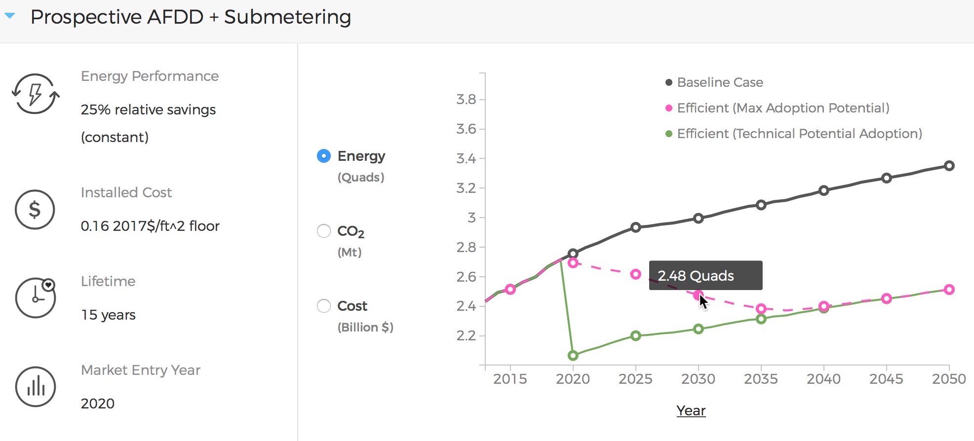
Fig. 1 Detailed data for a prospective AFDD ECM include key input attributes (at left) and primary energy use, CO₂ emissions, or energy cost results for the ECM under three ECM adoption scenarios (at right). In the energy use plot shown for this ECM, baseline primary energy use gradually increases across the modeled time horizon from 2.5 quads in 2015 to 3.35 quads in 2050; the ECM is ultimately able to reduce this baseline energy by more than 0.75 quads. The full impact of the ECM on baseline energy use is seen upon market entry in 2020 under a Technical Potential adoption scenario and by about 2040 under a Maximum Adoption Potential scenario.

Plots in the detailed ECM view show projected primary energy use, CO₂ emissions, or energy costs for the ECM under three ECM adoption scenarios (see ECMs are adopted one of two ways for more details on ECM adoption):

1. a “Baseline” technology case where no ECM adoption is assumed, corresponding to AEO Reference Case outcomes,

2. a “Technical Potential” case where the ECM is assumed to entirely replace comparable baseline technologies upon market entry, and

3. a “Maximum Adoption Potential” case where the ECM’s penetration into its baseline market is limited by more realistic baseline technology stock turnover.

Each plot’s x axis shows the year range for the projections; the y axis can be toggled to show the energy use, CO₂, or cost outcome of interest.

Tip

To view y axis values associated with each point on the plot, mouse over the points of interest and the values will appear.

Note

Plotted results on the ECM Summaries Page are estimated for each ECM in isolation - e.g., no competition with other ECMs is accounted for.

Download or edit ECM definitions

To download an ECM definition on the ECM Summaries Page, click the “Download” icon (the down arrow) at the right end of the row for the ECM of interest — this icon is also found at the top right of the detailed drop down window for the ECM. An ECM JSON will be downloaded to your computer; this JSON can be added to the ./ecm_definitions folder in your Scout directory and used in subsequent analyses.

To edit the attributes of an ECM on the ECM Summaries Page, click the “Edit” icon (the pencil) at the right right end of the row for the ECM of interest — this icon is also found at the top right of the detailed drop down window for the ECM.

An “Edit ECM” form will pop up with fully populated input fields (see Creating a new ECM or ECM package for additional guidance on these fields). For edits to single ECMs, click through the navigation bar steps on the left side of the form and make changes to the input fields shown in each step; ECM package edits only have one step. When your edits are complete, click the “Generate ECM” button at the bottom right of the screen to download an edited ECM JSON definition; again, this JSON can be added to the ./ecm_definitions folder in your Scout directory and used in subsequent analyses.

Tutorial 3: Creating new custom analyses

The ECM Summaries Page also allows you to create new, custom analyses with existing or new ECMs.

Create a new analysis with one or more ECMs from the ECM Summaries page

To conduct a new analysis, first select one or more of the ECM definitions on the ECM Summaries Page by clicking on the checkboxes next to the ECMs, and then enter a name for your analysis in the “Enter Analysis Name” box at the bottom of the screen.

Before you click “Start New Analysis,” which will no longer be greyed out after you enter a name for your analysis, you will need to pick an analysis calculation method. There are three calculation methods you can choose from depending on whether you are interested in assessing source or site energy impacts:

1. Fossil Fuel Equivalence: One of two approaches for non-combustible source energy accounting, this methodology uses the average heat rate of fossil generators and assigns it as the heat rate for non-combustible renewable energy generation. This value is 9,510 BTU/kWh, or about 35% efficiency, and represents the source energy value of fossil generation that is displaced by renewable energy generation.

2. Captured Energy: The other approach assumes that the source energy of renewable energy generators is exactly equal to the electricity produced with no energy losses prior to transmission and distribution. It is equal to a heat rate of 3,412 BTU/kWh, or a conversion efficiency of 100%.

3. Site Energy: This approach assess impacts in terms of site energy rather than in terms of source energy (using one of the other two approaches).

Note

Neither of the source energy accounting methods is strictly more accurate than the other. Both are a matter of methodological choice related to the specific application. We recommend reviewing this methodological guidance for more information before making your choice.

After selecting one of these calculation methods, click “Start New Analysis,” and a pop-up box will indicate that the analysis has started and is running in the background. To view the analysis queue, hover your mouse over the queue icon where you will see an “Analysis Status” dropdown. Click on this dropdown to open an “Analysis Status” pane that shows your analysis is underway. When it is complete, you will see a new notification appear. The “Analysis Status” pane will now show your analysis has status “Completed”.

Using the analysis selection dropdown on the Analysis Results page

On the Analysis Results Page you can click the dropdown menu to show all completed and in-progress analyses. The pane will show the status, name, calculation method, and run date/time for each analysis. Next to each analysis, you will also see icons that allow you perform operations on the completed analyses:

• Clicking the green gear icon shows you the list of ECMs included in your analysis. If you wish to run a new analysis using all or a subset of these ECMs, you can use the checkboxes to select or deselect ECMs and then click “Next” to start a new analysis with a modified set of ECMs or with a different calculation method.

• Clicking on the blue download icon allows you to download in JSON format raw results from your analysis.

• Clicking on the blue edit icon allows you to rename the analysis.

• Clicking on the red delete icon allows you to delete the analysis.

Tutorial 4: Viewing and understanding outputs

The Analysis Results Page allows you to view interactive results visualizations for ECM analyses.

Energy, CO₂, cost, and financial metrics tabs

Results are organized by one of four outcome variables of interest - “Energy,” “CO₂,” “Costs,” and “Financial Metrics” - each of which is assigned a tab at the top of the page. Here, “Energy” signifies total primary energy use; “CO₂” and “Costs” signify the total CO₂ emissions and operating costs associated with the total primary energy use; and “Financial Metrics” cover various consumer and portfolio-level metrics of ECM cost effectiveness.

On each of the four tabs, summary statistics for the variable of interest are shown in a single line at the top of the page. All statistics correspond to a particular year range, which is shown in parentheses next to the title above the statistics. The year range can be changed using the “Year Range” boxes on the left-hand filter bar.

Tip

Entering an identical minimum and maximum year (e.g., 2020 to 2020) into “Year Range” yields annual results; otherwise, the “Energy,” “CO₂,” and “Costs” results are added across the specified year range, and the “Financial Metrics” results are averaged across the specified year range.

Summary statistics are tailored to each tab - for example, the statistics on the “Energy” tab begin with avoided energy use, while the statistics on the “CO₂” tab begin with avoided CO₂ emissions.

Each of the “Energy,” “CO₂,” and “Costs” tabs features two types of plots - a radar graph and a bar graph. Switch between these graph types using the “Radar” and “Bar” graph toggle towards the top right of these pages. The “Financial Metrics” tab features a single scatterplot type. Each of these visualizations is detailed further below.

Radar graphs

The radar graph on the Analysis Results Page groups total energy, CO₂, or cost results by end use, climate zone, or building class. The graph has several axes that emanate from a single point of origin; each axis represents a category for one of the three grouping variables. The magnitude of total energy, CO₂, or cost attributed to each category is represented by the distance of a point on the category’s axis from the axis origin. Fig. 2 shows an example radar graph for a portfolio of prospective and commercially available ECMs.

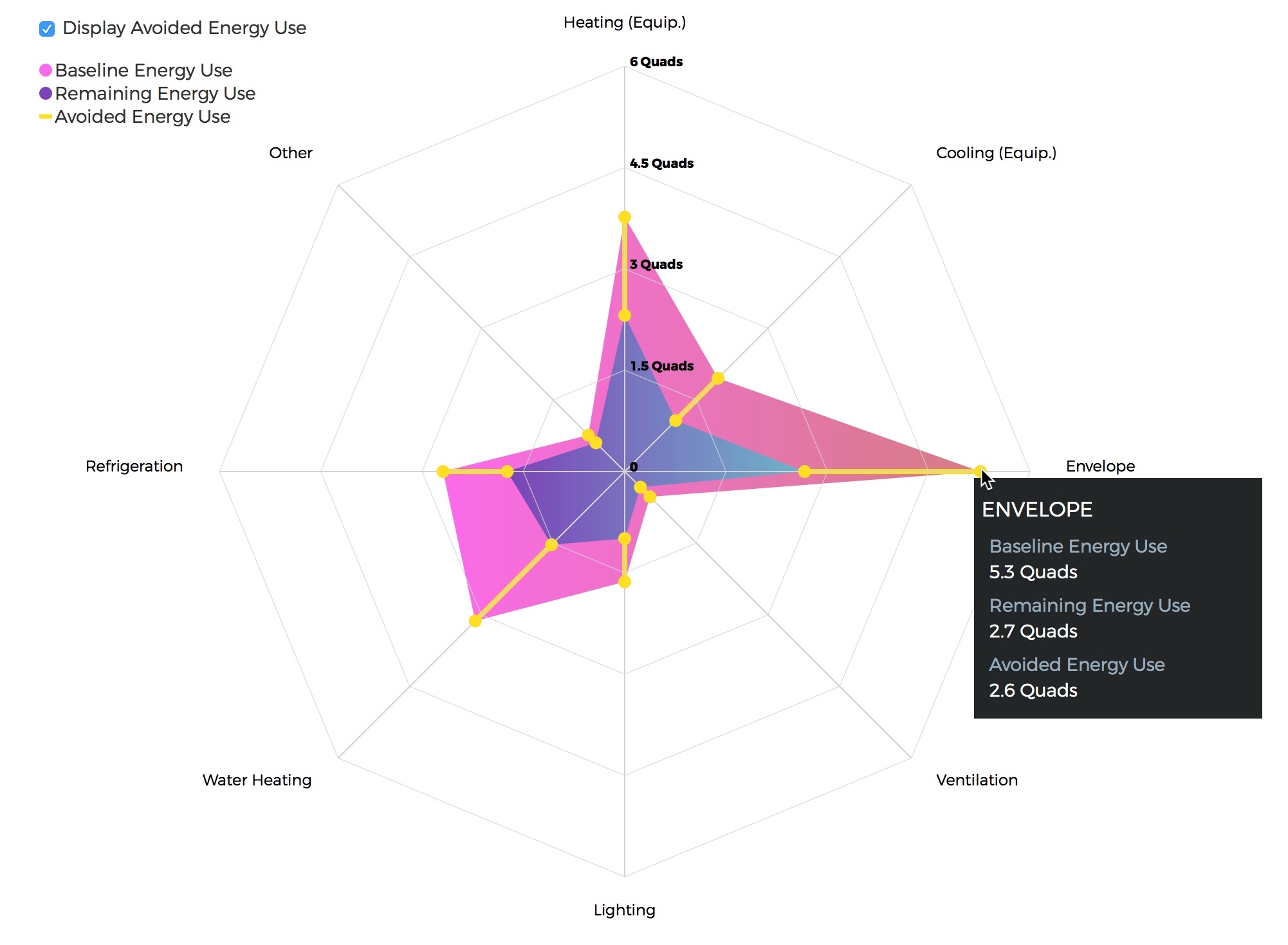
Fig. 2 In this radar graph, the overall primary energy use impact of an ECM portfolio that includes both prospective and commercially available ECMs is broken down by end use; results are shown for a Technical Potential adoption scenario run in the year 2030. Here, the envelope end use (pertaining to heating and cooling energy lost through building envelope components) makes the largest contribution to baseline energy use (5.3 quads) and ECM energy savings (2.6 quads). [2] Heating and water heating yield the second and third largest baseline energy use totals (3.8 and 3.1 quads, respectively); ECM energy savings are slightly higher for water heating than heating (1.6 quads water heating compared to 1.5 quads heating).

Results are shown for two energy use scenarios:

1. a “business-as-usual” case where no ECM adoption is assumed, corresponding to AEO Reference Case outcomes (titled “Baseline” on the plot and shaded pink), and

2. a case where at least some degree of ECM penetration into the baseline energy, CO₂, or cost market is assumed (titled “Remaining” on the plot and shaded purple).

Note

Comparing the pink and purple shaded polygons on each radar graph - corresponding to the “Baseline” and “Remaining” scenarios, respectively - yields a visual understanding of which categories make the greatest contributions to avoided energy use, CO₂, or cost.

Tip

To view more details about the avoided energy use, CO₂, or cost attributed to a particular category, mouse over the yellow points and connecting line shown along the category’s axis; a tooltip will appear that summarizes baseline, remaining, and avoided energy use, CO₂, or cost.

The yellow points and lines may be removed from the plot by unchecking the “Display Avoided Energy Use” box towards the top left of the plot region.

In scenario 2 (“Remaining”) where some degree of ECM market penetration is assumed, ECM adoption is simulated one of two ways:

1. “Technical Potential” adoption, where the ECM entirely replaces comparable baseline technologies upon market entry, or

2. “Maximum Adoption Potential”, where the ECM’s penetration into its baseline market is limited by realistic baseline technology stock turnover (see ECMs are adopted one of two ways for more details on ECM adoption).

Switch between the end use, climate zone, and building class grouping variables by selecting the appropriate radio button under the “Group By” label on the left-hand filter bar and clicking the “Apply Filter” button at the bottom of the filter bar.

Change ECM adoption assumptions by adjusting the radio button under the “Adoption Scenario” label in the left-hand filter bar and clicking “Apply Filter” at the bottom of the filter bar.

Bar graphs

The bar graph on the Analysis Results Page attributes total avoided energy, CO₂, or cost results to individual ECMs. The plot unfolds from left to right, beginning with a “Baseline” segment of energy use, CO₂, or cost that is broken into “Avoided” and “Remaining” segments; each of these segments is then further attributed to the individual ECMs. Fig. 3 shows an example bar graph for a portfolio of prospective and commercially available ECMs.

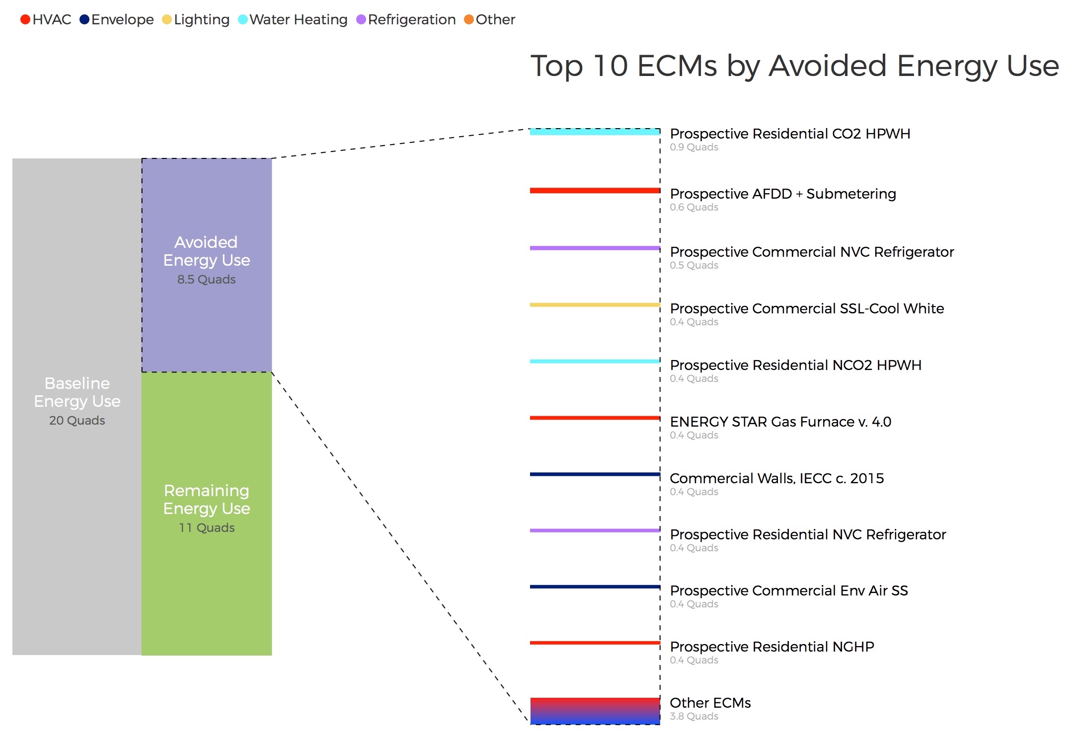
Fig. 3 This bar graph attributes total avoided and remaining energy use after ECM portfolio adoption to individual ECMs in the portfolio, grouping each ECM by the end use that it applies to. In this case, representing a Technical Potential ECM adoption run for the year 2030, two heat pump water heating (HPWH) ECMs appear in the top 5 ECM contributions to total avoided energy use. This result stems from the generally high potential for energy use impacts in the water heating end use (see Fig. 2) and the high performance levels of these HPWH ECMs relative to the baseline technologies they replace (here assumed to include gas-fired water heaters). Most of the ECMs on this list represent aspirational technologies with targeted cost and performance attributes.

Tip

Clicking on the “Avoided” and “Remaining” segment bars shows the individual ECM contributions to each of these segments.

The magnitude of each ECM’s contribution to the “Avoided” and “Remaining” bar segments is indicated in three ways:

1. by the ECM’s vertical position on the list of individual ECMs, with more impactful ECMs shown higher on the list, and

2. by the height of each ECM’s corresponding bar segment, and

3. by the specific energy, CO₂, or cost impact noted under the ECM’s name label.

ECM bar segments may be color-coded by end use, climate zone, and building class; select the appropriate radio button under the “Group By” label on the left-hand filter bar and click the “Apply Filter” button at the bottom of the filter bar.

ECM bar segments may also be filtered by end use, climate zone, and building class by checking the appropriate box(es) under the “End Uses,” “Climate Zones,” and/or “Building Class” labels on the left-hand filter bar and clicking the “Apply Filter” button at the bottom of the filter bar.

As for the ECM Summaries Page, previous ECM filter selections are cleared by clicking the “Clear All” text at the bottom of the filter bar; the filter bar may also be hidden by clicking the left-pointing arrow shown at the top right of the bar.

Scatterplots

The scatterplot on the Analysis Results Page indicates the cost effectiveness of individual ECMs under multiple financial metrics - Internal Rate of Return (IRR), Simple Payback, Cost of Conserved Energy, and Cost of Conserved Carbon - each of which may be assigned to the x or y axis of the plot using adjacent dropdown menus. Fig. 4 shows an example scatterplot for a portfolio of prospective and commercially available ECMs.

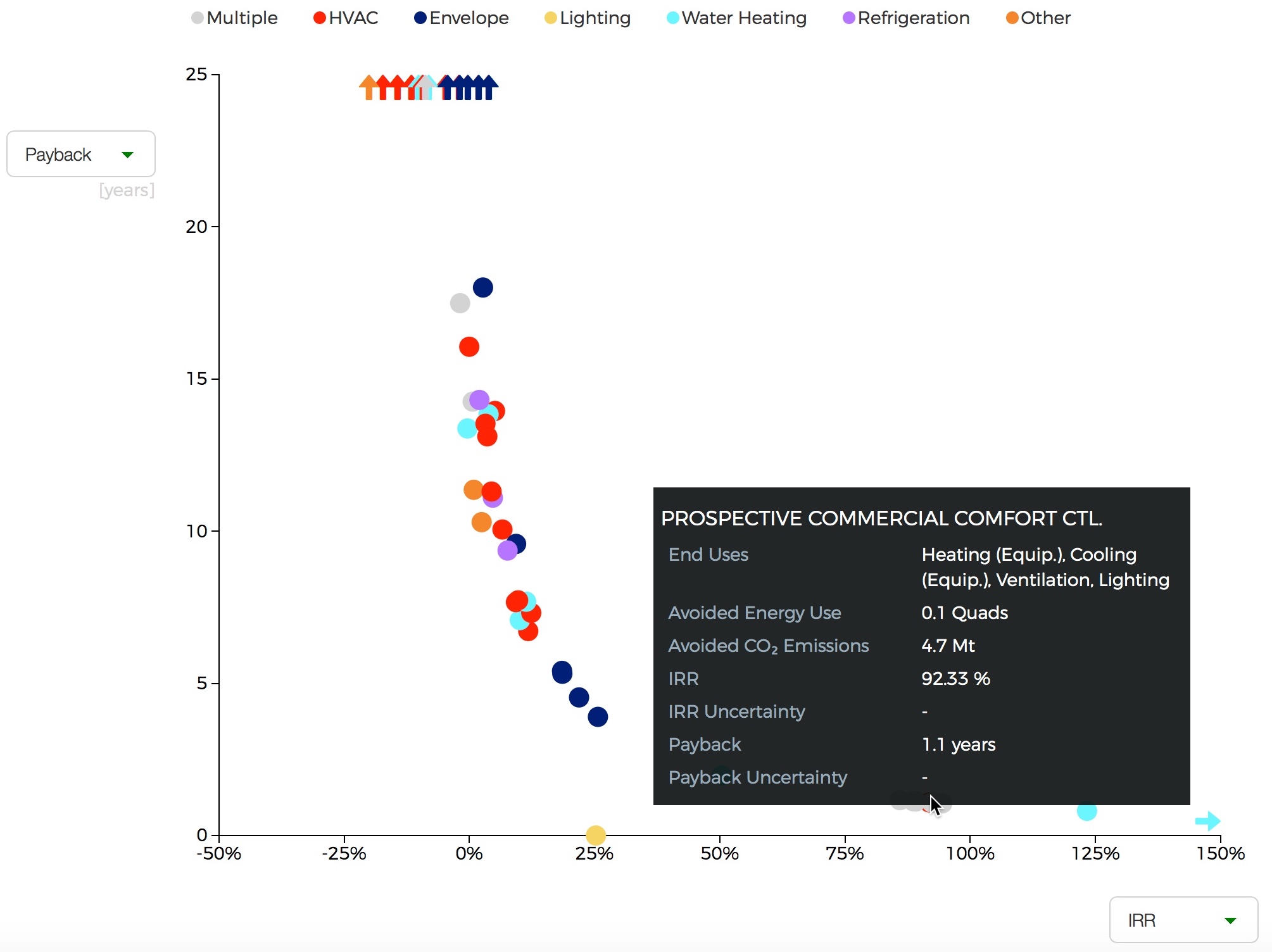
Fig. 4 This scatterplot indicates the cost effectiveness of individual ECMs under two financial metrics, grouping ECMs by the end use(s) they apply to. In this case, representing a Technical Potential ECM adoption run for the year 2030, internal rate of return (IRR) and simple payback financial metrics are used on the x and y axes, respectively. ECMs toward the bottom right of the plot (lower payback, higher IRR) are most cost effective. Most ECMs in the plot region below 5 years payback and above an IRR of 10% apply to the envelope, water heating, or “Multiple” end use categories, where the latter category reflects controls ECMs. Controls ECMs look particularly favorable here since their targeted cost and performance attributes were developed under a more aggressive payback requirement than other ECM types (~1 year). For example, the highlighted “Commercial Comfort Ctl.” ECM yields a 1.1 year payback in 2030, though this ECM only saves 0.1 quads of energy because its application was restricted to large offices for this run.

Note

For all of the financial metrics except for IRR, a higher number signifies lower ECM cost effectiveness.

ECM points on the scatterplot may be color-coded by end use, climate zone, and building class; select the appropriate radio button under the “Group By” label on the left-hand filter bar and click the “Apply Filter” button at the bottom of the filter bar.

ECM points may also be filtered by end use, climate zone, and building class by checking the appropriate box(es) under the “End Uses,” “Climate Zones,” and/or “Building Class” labels on the left-hand filter bar and clicking the “Apply Filter” button at the bottom of the filter bar.

Tip

To see more details about an ECM’s avoided energy use and CO₂ emissions, as well as the financial metric outcomes for an ECM under the current axis selections, hover your cursor over the ECM point of interest; a tooltip will appear with these details.

If a probability distribution has been placed on the cost, performance, and/or lifetime input(s) of one or more ECMs, uncertainty in the resultant cost effectiveness of any affected ECMs is expressed as a lightly shaded region around the affected ECM points on the scatterplot. Uncertainty ranges are also reported around the financial metric results in the detail tooltips of affected ECMs.

Tutorial 5: Using the Baseline Energy Calculator

The Baseline Energy Calculator allows you to determine the total energy and CO₂ impact potential of an individual ECM or group of ECMs, drawing data from the Energy Information Administration’s Annual Energy Outlook (AEO).

The Calculator guides you through four steps to determining the total baseline energy use or CO₂ emissions associated with a particular market segment, shown below.

All inputs to the Baseline Energy Calculator form are required unless they are tagged “optional”. Refer to red error messages below missing input(s) to ensure that your entries are complete.

1. Select an AEO version year. Click the dropdown menu next to “AEO Year” to select which version of the EIA AEO you would like to use in generating results.

2. Select a projection year. Click the dropdown menu to select the year for which baseline energy or CO₂ emissions estimates are desired. Note: past years represent historical EIA estimates.

3. Select relevant climate zone(s). Climate zone(s) are selected by checking the appropriate box(es) or by clicking the region(s) of interest on the map. An “All” selection will automatically check all of the climate zone sub-categories.

Note

Scout currently uses the AIA climate zone breakdowns from RECS 2009 and CBECS 2003.

4. Select building type(s). Building type(s) are selected by checking the appropriate box(es). An “All Residential” or “All Commercial” selection will automatically check all residential and commercial building sub-categories, respectively.

Tip

Both residential and commercial building types may be selected simultaneously if you are interested in understanding impact potential across the entire buildings sector. [3]

5. Select end use(s) and technology type(s). End use(s) are selected by clicking the drop down menu bar and checking the appropriate box(es); click the drop down bar again to hide your end use selections and move on to subsequent selections. After most end use selections, a “Fuel Type” input will appear; upon selecting fuel type(s), a final “Technology” input will appear. [4]

Once all steps of the Baseline Energy Calculator have been completed, click the “Calculate” button at the bottom right of the screen to obtain the energy use and associated CO₂ emissions results.

Tip

Initial results may cleared by clicking the “Reset” button or updated by clicking the “Calculate” button again.

Footnotes

[1]

In the special case of a “Heating,” “Secondary Heating,” and/or “Cooling” end use selection, an additional “Technology Type” input will appear, as heating/cooling technologies may be categorized as equipment (e.g., an efficient air source heat pump) or as envelope components (e.g., a highly insulating window). Choosing “Equipment” as the “Technology Type” will yield subsequent “Fuel Type” and “Technology” inputs. Choosing “Envelope” as the “Technology Type” skips the “Fuel Type” input and moves you straight to the “Technology” input; this reflects that the energy use associated with envelope components is not tied to a specific fuel type.

[2]

EnergyPlus Measure performance data are always provided with units of relative savings.

[3]

Envelope energy use totals in Fig. 2 reflect simultaneous improvements in the efficiency of the heating and cooling equipment and lighting end uses (contributing 3.8, 2.0, and 1.6 quads of baseline energy use, respectively).

[4]

When both residential and commercial buildings are selected in step 3, subsequent end use and technology selections in step 4 will reflect both of these sectors. For example, in the end use dropdown menu, both “Secondary Heating” (residential only) and “Ventilation” (commercial only) end uses will be shown, while in the technology dropdown menu, “Wood Stove” (residential only) and “Engine-driven Heat Pump” (commercial only) will be shown.

[5]

In the special case of a “Heating,” “Secondary Heating,” and/or “Cooling” end use selection, an additional “Equipment” and “Envelope” toggle will appear, as heating/cooling technologies may be categorized as equipment (e.g., an efficient air source heat pump) or as envelope components (e.g., a highly insulating window). Toggling “Equipment” will yield subsequent “Fuel Type” and “Technology” inputs. Toggling “Envelope” as the “Technology Type” skips the “Fuel Type” input and moves you straight to the “Technology” input; this reflects that the energy use associated with envelope components is not tied to a specific fuel type.