Local Execution Tutorials
Tutorial 1: Creating and editing ECMs
Before beginning this tutorial, it is recommended that you review the list of parameters in an ECM definition.
The ECM JSON schema should always be in your back pocket as a reference. This section includes brief descriptions, allowable options, and examples for each of the fields in an ECM definition. You might want to have it open in a separate tab in your browser while you complete this tutorial, and any time you’re authoring or editing an ECM.
The example in this tutorial will demonstrate how to write new ECMs so that they will be compliant with all relevant formatting requirements and provide the needed information about a technology in the structure expected by the Scout analysis engine. This example is intentionally plain to illustrate the basic features of an ECM definition and is not an exhaustive description of all of the detailed options available to specify an ECM. These additional options are presented in the Additional ECM features section, and the ECM JSON schema has detailed specifications for each field in an ECM definition. In addition, this tutorial includes information about how to edit existing ECMs and define package ECMs.
As a starting point for writing new ECMs, an empty ECM definition file is available for download. Reference versions of the tutorial ECMs are also provided for download to check one’s own work following completion of the examples.
Each new ECM created should be saved in a separate file. To add new or edited ECMs to the analysis, the files should be placed in the ./ecm_definitions directory, or in a directory specified by the user. Further details regarding where ECM definitions should be saved and how to ensure that they are included in new analyses are included in Tutorial 3.
JSON syntax basics
Each ECM for Scout is stored in a JSON-formatted file. JSON files are human-readable (they appear as plain text) and are structured as (nested) pairs of keys and values, separated by a colon and enclosed with braces. [1]
{"key": "value"}
Warning
JSON files have important formatting rules that must be strictly observed. JSON files that do not follow these rules are “invalid” and cannot be used by any program.
Keys are always text – both letters and numbers are acceptable – enclosed in double quotes. Values can take one of several forms, such as numbers, boolean values (i.e., true, false), or lists (multiple values separated by commas and enclosed in brackets). A value must always be provided for each key.
{"temperature": 450}
{"activated": true}
{"preferred colors": ["red", "green", "blue"]}
{"reported heights": [1.79, 1.83, 1.64, 1.91]}
There can be multiple key-value pairs at the same level, separated by commas.
{"name": "HAL", "model": 9000, "service date": "1992-01-12"}
Values can also be additional key-value pairs, thus creating a nested structure.
{"vehicle 1": {"make": "Ford", "model": "F-150"}}
{"name": "HAL", "model": 9000, "service date": "1992-01-12",
 "manufacturing location": {"country": "US", "state": "IL", "city": "Urbana"}}
Among key-value pairs at the same level, the order of entries does not matter.
We will use these formatting guidelines to write new ECMs.
Your first ECM definition
The required information for defining this ECM will be covered in the same order as the list of parameters in the Analysis Approach section. For all of the fields in the ECM definition, details regarding acceptable values, structure, and formatting are provided in the ECM JSON schema.
If after completing this tutorial you feel that you would benefit from looking at additional ECM definitions, you can browse the :repo_file:`ECM definition JSON files <ecm_definitions>` available on GitHub.
For this example, we will be creating an ECM for LED troffers for commercial buildings. Troffers are square or rectangular light fixtures designed to be used in a modular dropped ceiling grid commonly seen in offices and other commercial spaces.
The finished ECM specification is available to download for reference.
To begin, the ECM should be given a descriptive name less than 40 characters long (including spaces). Details regarding the characteristics of the technology that will be included elsewhere in the ECM definition, such as the cost, efficiency, or lifetime, need not be included in the name. The key for the name is simply name.
{"name": "LED Troffers"}
If the ECM describes a technology currently under development, the name should contain the word “Prospective” in parentheses. If the ECM describes or is derived from a published standard or specification, its version number or year should be included in the name.
Note
In this tutorial, JSON entries will be shown with leading and trailing ellipses to indicate that there is additional data in the ECM definition that appears before and/or after the text of interest.
{...
 "key_text": "value",
 ...}
Applicable baseline market
The applicable baseline market parameters specify the climate zones, building types, structure types, end uses, fuel types, and specific technologies for the ECM.
The climate zone(s) can be given as a single string, if only one climate zone applies, or as a list if a few climate zones apply. The climate zone entry options are outlined in the Climate zone section, and formatting details are in the applicable section of the JSON schema. If the ECM is suitable for all climate zones, the shorthand string "all" can be used in place of a list of all of the climate zone names. These shorthand terms are discussed further in the Baseline market shorthand values section.
LED troffers can be installed in buildings in any climate zone, and for convenience, the available shorthand term will be used in place of a list of all of the climate zone names.
{...
 "climate_zone": "all",
 ...}
Building type options include specific residential and commercial building types, given in the Building type section, as well as several shorthand terms. A single string, list of strings, or shorthand value(s) are all allowable entries, as indicated in the bldg_type field reference.
Though LED troffers are most commonly found in office and other small commercial settings, they are found to some limited extent in most types of commercial buildings. Rather than limiting the ECM to only some building types, the technology field will be used to restrict the applicability of the ECM to only the energy used by lighting types that could be replaced by LED troffers.
{...
 "bldg_type": "all commercial",
 ...}
ECMs can apply to only new construction, only existing buildings, or all buildings both new and existing. This is specified under the structure_type key with the values “new,” “existing,” or “all,” respectively.
LED troffers can be installed in both new construction and existing buildings, thus the “all” shorthand is used.
{...
 "structure_type": "all",
 ...}
The end use(s) correspond to the major building functions or other energy uses provided by the technology described in the ECM. End uses can be specified as a single string or, if multiple end uses apply, as a list. The acceptable formats for the end use(s) are in the ECM JSON schema and the acceptable values are listed in the End use ECM reference section. [2] If the ECM describes a technology that affects the thermal load of a building (e.g., insulation), the end use should be given as “heating” and “cooling” in a list.
The only applicable end use for LED troffers is lighting. Changing from fluorescent bulbs typically found in troffers to LEDs will reduce the heat output from the fixture, thus reducing the cooling load and increasing the heating load for the building. These changes in heating and cooling energy use that arise from changes to lighting systems in commercial buildings are accounted for automatically in the energy use calculations for the ECM.
{...
 "end_use": "lighting",
 ...}
The fuel type generally corresponds to the energy source used for the technology described by an ECM – natural gas for a natural gas heat pump and electricity for an air-source heat pump, for example. The fuel type should be consistent with the end use(s) already specified, based on the end use reference tables. Fuel types are listed in the Fuel type ECM reference section, and can be specified as a single entry or a list if multiple fuel types are relevant (as indicated in the ECM JSON schema). If the ECM describes a technology that affects the thermal load of a building (e.g., insulation), the fuel type should be given as “all” because heating and cooling energy from all fuel types could be affected by those types of technologies.
In the case of LED troffers, electricity is the only relevant fuel type.
{...
 "fuel_type": "electricity",
 ...}
The technology field drills down into the specific technologies or device types that apply to the end use(s) for the ECM. In some cases, an ECM might be able to replace the full range of incumbent technologies in its end use categories, while in others, only specific technologies might be subject to replacement. As indicated in the ECM JSON schema, applicable technologies can be given as a single string, a list of technology names, or using shorthand values. If applicable, a technology list can also be specified with a mix of shorthand end use references (e.g., “all lighting”) and specific technology names, such as ["all heating", "F28T8 HE w/ OS", "F28T8 HE w/ SR"].
All of the technology names are listed by building sector (residential or commercial) and technology type (supply or demand) in the relevant section of the ECM Definition Reference. In general, the residential and commercial thermal load components are the technology names for demand-side energy use, and are relevant for ECMs that apply to the building envelope or windows. Technology names for supply-side energy use generally correspond to major equipment types used in the AEO [3] and are relevant for ECMs that are describing those types of equipment within a building.
For this example, LED troffers are likely to replace linear fluorescent bulbs, the typical bulb type in troffers. There are many lighting types for commercial buildings, but we will include all of the lighting types that are specified as T__F__, which correspond to linear fluorescent bulb types, including those with additional modifying text.
{...
 "technology": ["T5 F28", "T8 F28 High-efficiency/High-Output", "T8 F32 Commodity", "T8 F59 High Efficiency", "T8 F59 Typical Efficiency", "T8 F96 High Output"],
 ...}
Market entry and exit year
The market entry year represents the year the technology is or will be available for purchase and installation. Some ECMs might be prospective, representing technologies not currently available. Others might represent technologies currently commercially available. The market entry year should reflect the current status of the technology described in the ECM. Similarly, the market exit year represents the year the technology is expected to be withdrawn from the market. If the technology described by an ECM will have a lower installed cost or improved energy efficiency after its initial market entry, another ECM should be created that reflects the improved version of the product, and the market exit year should not (in general) be used to force an older technology out of the market.
The market entry year and exit year both require source information. As much as is practicable, a high quality reference should be used for both values. If no source is available, such as for a technology that is still quite far from commercialization, a brief explanatory note should be provided for the market entry year source, and the source_data fields themselves can be given as null or with empty strings. If it is anticipated that the product will not be withdrawn from the market prior to the end of the model time horizon, the exit year and source should be given as null.
LED troffers are currently commercially available with a range of efficiency, cost, and lifetime ratings. It is likely that while LED troffers will not, in general, exit the market within the model time horizon, LED troffers with cost and efficiency similar to this ECM are not likely to remain competitive through 2040. It will, however, be left to the analysis to determine whether more advanced lighting products enter the market and supplant this ECM, rather than specifying a market exit year.
{...
 "market_entry_year": 2015,
 "market_entry_year_source": {
   "notes": "The source suggests that technologies described in the document are available on the market by its release date.",
   "source_data": [{
      "title": "High Efficiency Troffer Performance Specification, Version 5.0",
      "author": "",
      "organization": "U.S. Department of Energy",
      "year": 2015,
      "pages": null,
      "URL": "https://betterbuildingssolutioncenter.energy.gov/sites/default/files/attachments/High%20Efficiency%20Troffer%20Performance%20Specification.pdf"}]},
 "market_exit_year": null,
 "market_exit_year_source": null,
 ...}
Energy efficiency
The energy efficiency of the ECM must be specified in three parts: the quantitative efficiency (only the value(s)), the units of the efficiency value(s) provided, and source(s) that support the indicated efficiency information. Each of these parameters is specified in a separate field.
The units specified are expected to be consistent with the units for each end use outlined in the ECM Definition Reference section.
The source(s) for the efficiency data should be credible sources, such as those outlined in the Analysis Approach section. The source information should be provided using only the fields shown in the example and should include sufficient information so that the value(s) can be quickly identified from the sources listed. Additional detail regarding the acceptable form for entries in the source are linked to from the source_data entry in the ECM JSON schema.
For the example of LED troffers, all lighting data should be provided in the units of lumens per Watt (denoted “lm/W”). LED troffers efficiency information is based on the High Efficiency Troffer Performance Specification.
{...
 "energy_efficiency": 120,
 "energy_efficiency_units": "lm/W",
 "energy_efficiency_source": {
   "notes": "Initial efficiency value taken from source section II.a.2.a. Efficiency value increased slightly based on efficacy values for fixtures categorized as '2x4 Luminaires for Ambient Lighting of Interior Commercial Spaces' in the DesignLights Consortium Qualified Products List (https://www.designlights.org/qpl).",
   "source_data": [{
      "title": "High Efficiency Troffer Performance Specification, Version 5.0",
      "author": "",
      "organization": "U.S. Department of Energy",
      "year": 2015,
      "pages": 5,
      "URL": "https://betterbuildingssolutioncenter.energy.gov/sites/default/files/attachments/High%20Efficiency%20Troffer%20Performance%20Specification.pdf"}]},
 ...}
Many additional options exist that enable more complex definitions of energy efficiency, such as incorporating probability distributions, providing a detailed efficiency breakdown by elements of the applicable baseline market, and using relative instead of absolute units. Detailed examples for all of the options are in the Additional ECM features section.
Installed cost
The absolute installed cost must be specified for the ECM, including the cost value, units, and reference source. The cost units should be specified according to the relevant section of the ECM Definition Reference, noting that residential and commercial equipment have different units, and that sensors and controls ECMs also have different units from other equipment types. The source information should be provided using the same keys and structure as the energy efficiency source. For ECMs that describe technologies not yet commercialized, assumptions incorporated into the installed cost estimate should be described in the notes section of the source.
If applicable to the ECM, separate cost values can be provided by building type and structure type, as described in the Detailed input specification section. Probability distributions can also be used instead of point values for the cost, using the format outlined in the Probability distributions section.
For LED troffers, costs are estimated based on an assumption of a single fixture providing 4800 lm, with installation requiring two hours and two people at a fully-burdened cost of $100/person/hr. The assumptions are articulated using the notes key under the installed_cost_source key.:
{...
 "installed_cost": 233.33,
 "cost_units": "$/1000 lm",
 "installed_cost_source": {
   "notes": "Assumes single fixture provides 4800 lm; requires 2 hour install with 2 people at a fully-burdened cost of $100/person/hr. Luminaire cost based on a range of retail prices found for luminaires with similar specifications found online in October 2016.",
   "source_data": [{
      "title": "",
      "author": "",
      "organization": "",
      "year": null,
      "pages": null,
      "URL": ""}]},
 ...}
Lifetime
The lifetime of the ECM, or the expected amount of time that the ECM technology will last before requiring replacement, is specified using a structure identical to the installed cost. Again, the lifetime value, units, and source information must be specified for the corresponding keys. The product lifetime can also be specified with a probability distribution and/or different values by building type. The units should always be in years, ideally as integer values greater than 0. The source information follows the same format as for the energy efficiency and installed cost. For ECMs that describe technologies not yet commercialized, assumptions in the lifetime estimate should be explained in the notes section of the source.
LED troffers have rated lifetimes on the order of 50,000 hours, though the High Efficiency Troffer Performance Specification requires a minimum lifetime of 68,000 hours. The values for lighting lifetimes should be based on assumptions regarding actual use conditions (i.e., number of hours per day), and the notes value in the source specification should include that assumption. The LED troffers in this example are assumed to operate 12 hours per day.
{...
 "product_lifetime": 15,
 "product_lifetime_units": "years",
 "product_lifetime_source": {
   "notes": "Calculated from 68,000 hrs, stated as item II.c.i, assuming 12 hr/day operation.",
   "source_data": [{
      "title": "High Efficiency Troffer Performance Specification, Version 5.0",
      "author": "",
      "organization": "U.S. Department of Energy",
      "year": 2015,
      "pages": 5,
      "URL": "https://betterbuildingssolutioncenter.energy.gov/sites/default/files/attachments/High%20Efficiency%20Troffer%20Performance%20Specification.pdf"}]},
 ...}
Other fields
The measure_type field indicates whether an ECM directly replaces the service of an existing device or building component or improves the efficiency of an existing technology. Examples include a cold-climate heat pump replacing existing electric heating and cooling systems and a window film that decreases solar heat gain, respectively. Further discussion of how to use the measure_type field and illustrative examples are in the Add-on type ECMs section.
LED troffers would replace existing troffers that use linear fluorescent bulbs, providing an equivalent building service (lighting) using less energy. The LED troffers ECM is thus denoted as “full service.”
{...
 "measure_type": "full service",
 ...}
If the ECM is intended to replace baseline technologies of a different technology and/or fuel type, the technologies and fuel types that it switches away from are specified in the technology and fuel_type fields, respectively, and the technology and fuel type that the ECM switches to are specified in the tech_switch_to and fuel_switch_to fields, respectively. These fields are explained further, with illustrative examples in the Technology and/or fuel switching section. When not applicable, the tech_switch_to and fuel_switch_to fields should be given the value null.
The LED troffers ECM switches away from linear fluorescent bulbs but does not switch fuels.
{...
 "fuel_switch_to": null,
 "tech_switch_to": "LED",
  ...}
If the ECM applies to only a portion of the energy use in an applicable baseline market, even after specifying the particular end use, fuel type, and technologies that are relevant, a scaling value can be added to the ECM definition to specify what fraction of the applicable baseline market is truly applicable to that ECM.
When creating a new ECM, it is important to carefully specify the applicable baseline market to avoid the use of the market scaling fraction parameter, if at all possible. If the scaling fraction is not used, the value and the source should be set to null. Details regarding the use of the market scaling fraction can be found in the Market scaling fractions section.
No market scaling fraction is required for the LED troffers ECM.
{...
 "market_scaling_fractions": null,
 "market_scaling_fractions_source": null,
 ...}
Two keys are provided for ECM authors to provide additional details about the technology specified. The _description field should include a one to two sentence description of the ECM, including additional references for further details regarding the technology if it is especially novel or unusual. The _notes field can be used for explanatory notes regarding the technologies that are expected to be replaced by the ECM and any notable assumptions made in the specification of the ECM not captured in another field.
{...
 "_description": "LED troffers for commercial modular dropped ceiling grids that are a replacement for the entire troffer luminaire for linear fluorescent bulbs, not a retrofit kit or linear LED bulbs that slot into existing troffers.",
 "_notes": "Energy efficiency is specified for the luminaire, not the base lamp.",
 ...}
Basic contact information regarding the author of a new ECM should be added to the fields under the _added_by key.
{...
 "_added_by": {
   "name": "Carmen Sandiego",
   "organization": "Super Appliances, Inc.",
   "email": "carmen.sandiego@superappliances.com",
   "timestamp": "2015-07-14 11:49:57 UTC"},
 ...}
When updating an existing ECM, the identifying information for the contributor should be provided in the _updated_by field instead of the “_added_by” field. If the ECM is new, the child keys in the “_updated_by” section should be given null values.
{...
 "_updated_by": {
   "name": null,
   "organization": null,
   "email": null,
   "timestamp": null},
 ...}
The LED troffers ECM that you’ve now written can be simulated with Scout by following the steps in subsequent tutorials. Many technologies will have ECM definitions like the one you just created, but some technologies, like sensors and controls and windows and opaque envelope products, will have definitions that are subtly different. Sensors and controls ECMs augment the efficiency of existing equipment in the stock, rather than replacing existing and supplanting new equipment. To get a feel for what these types of add-on technologies look like as an ECM, you can download and review an Automated Fault Detection and Diagnosis (AFDD) ECM. Additional information about sensors and controls ECMs can be found in the Add-on type ECMs section. Windows and opaque envelope technologies reduce demand for heating and cooling instead of increasing the efficiency of the supply of heating and cooling. An ECM for the ENERGY STAR windows version 6 specification is available to download to illustrate demand-reducing ECMs.
Additional ECM features
There are many ways in which an ECM definition can be augmented, beyond the basic example already presented, to more fully characterize a technology. The subsequent sections explain how to implement the myriad options available to add more detail and complexity to your ECMs. Links to download example ECMs that illustrate the feature described are included in each section.
Technology and/or fuel switching
Example – Heat Pump Water Heater (Details)
Some ECMs switch a comparable baseline technology to a different technology and/or fuel type. Air or ground source heat pumps, for example, can replace the service of fossil-fired heating systems (different fuel, different technology), or these heat pumps can replace the service of electric resistance baseboard heaters or furnaces (same fuel, different technology). The same goes for heat pump water heaters and for electric ranges and dryers. The tech_switch_to field, used in conjunction with the technology field and the fuel_type and fuel_switch_to fields in the baseline market, enables an ECM to replace the service of a different baseline technology and/or fuel type.
To configure such ECMs, the technology and fuel_type fields should be populated with a list of the technologies and fuel types that, for the applicable end uses, are replaced by the ECM technology. If the ECM is able to replace all technologies for a given fuel type and end use, the technology field can be specified using the "all" shorthand value. The tech_switch_to field should be set to the most appropriate value for the ECM from Table 1, while the fuel_switch_to field should be set to ECM fuel type being switched to.
ECM Technology Switched To |
JSON Value |
|---|---|
Air source heat pump |
|
Ground source heat pump |
|
Heat pump water heater |
|
Electric cooking |
|
Electric drying |
|
LED |
|
For example, an air source heat pump ECM could replace the service of fossil-fired furnaces paired with central air conditioners.
{...
 "fuel_type": ["natural gas", "distillate", "electricity"],
 ...
 "technology": ["furnace (NG)", "furnace (distillate)", "central AC"],
 ...
 "fuel_switch_to": "electricity",
 "tech_switch_to": "ASHP",
 ...}
Alternatively, an air source heat pump ECM could replace the service of electric resistance furnaces paired with central air conditioning.
{...
 "fuel_type": ["electricity"],
 ...
 "technology": ["resistance heat", "central AC"],
 ...
 "fuel_switch_to": null,
 "tech_switch_to": "ASHP",
 ...}
Note
The ecm_prep.py module checks for and expects tech_switch_to information for all fuel switching and LED measures (“LED”, “solid state”, “Solid State”, or “SSL” in name), as well as for heat pump measures (“HP”, “heat pump”, or “Heat Pump” in name) that apply to electric resistance heating or water heating technologies in the baseline. The ecm_prep.py execution will error if this expected information is missing. If a measure meeting those criteria is not intended to represent technology switching, the user can suppress this check by setting the measure’s tech_switch_to to value null.
A residential heat pump water heater is available to download to illustrate the setup of the tech_switch_to, fuel_switch_to, technology, and fuel_type fields to denote, for this particular example, an electric water heater that can replace water heaters of fossil-fired fuel types.
Time sensitive valuation
In certain cases, ECMs might affect baseline energy loads differently depending on the time of day or season, necessitating time sensitive valuation of ECM impacts. Fig. 5 demonstrates three possible types of time sensitive ECM features.
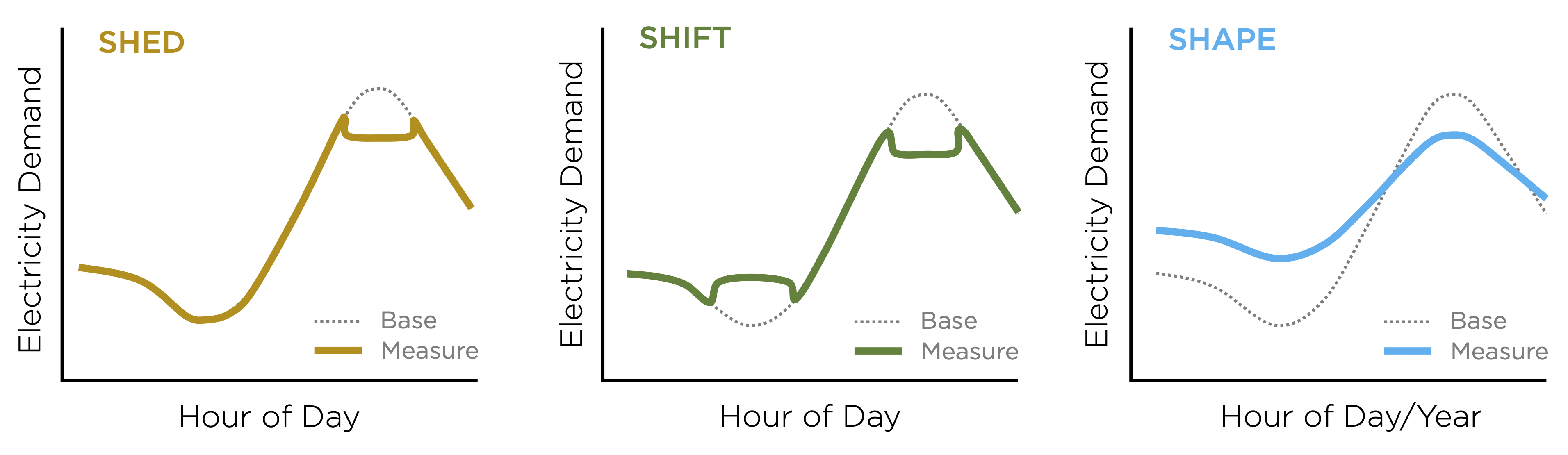
Fig. 5 Time sensitive ECM features include (from left): load shedding, where an ECM reduces load during a certain daily hour range; load shifting, where load is reduced during one daily hour range and increased during another daily hour range; and load shaping, where load may be increased or decreased for any hour of the day/year in accordance with a custom hourly load savings shape.
Such time sensitive ECM features are specified using the tsv_features parameter, which adheres to the following general format:
{...
 "tsv_features": {
   <time sensitive feature>: {<feature details>}},
 ...}
The tsv_features parameter may be broken out by an ECM’s climate_zone, bldg_type, and/or end_use:
{...
 "tsv_features": {
   <region 1> : {
     <building type 1> : {
       <end use 1>: {
         <time sensitive feature>: {<feature details>}}}}, ...
   <region N> : {
     <building type N> : {
       <end use N>: {
         <time sensitive feature>: {<feature details>}}}}},
 ...}
Source information for time sensitive ECM features is specified using the tsv_source parameter:
{...
 "tsv_source": {
   "notes": <notes>,
   "source_data": [{
     "title": <title>,
     "author": <author>,
     "organization": <organization>,
     "year": <year>,
     "pages":[<start page>, <end page>],
     "URL": <URL>}]},
 ...}
The tsv_source parameter may be broken out by an ECM’s climate_zone, bldg_type, and/or end_use, and by the ECM’s time sensitive valuation features:
{...
 "tsv_source": {
   <region 1> : {
       <building type 1> : {
         <end use 1>: {
           <time sensitive feature>: {
             "notes": <notes>,
             "source_data": [{
               "title": <title>,
               "author": <author>,
               "organization": <organization>,
               "year": <year>,
               "pages":[<start page>, <end page>],
               "URL": <URL>}]}}}}, ...
   <region N> : {
       <building type N> : {
         <end use N>: {
           <time sensitive feature>: {
             "notes": <notes>,
             "source_data": [{
               "title": <title>,
               "author": <author>,
               "organization": <organization>,
               "year": <year>,
               "pages":[<start page>, <end page>],
               "URL": <URL>}]}}}},
 ...}
Each time sensitive ECM feature is further described below with illustrative example ECMs.
Note
Time sensitive ECM features are currently only supported for ECMs that affect the electric fuel type across the 2019 EIA Electricity Market Module (EMM) regions, and may not be defined as fuel switching measures.
Accordingly, when preparing an ECM with time sensitive features, the user should ensure that:
the ECM’s fuel_type parameter is set to
"electricity", and the ECM’s fuel_switch_to parameter is set tonull;ecm_prep.py is executed with the
--alt_regionsoption specified; andEMM is subsequently selected as the alternate regional breakout.
Users are also encouraged to use the --site_energy option when executing ecm_prep.py for ECMs with time sensitive features, as utility planners are often most interested in the change in the electricity demand (rather than generation) that may result from ECM deployment.
Note
The effects of an ECM’s time sensitive features are applied on top of the ECM’s static energy efficiency impact on baseline loads, as defined in the ECM’s energy_efficiency parameter.
Example – Commercial AC (Shed) ECM (Details)
The first type of time sensitive ECM feature sheds (reduces) a certain percentage of baseline electricity demand (defined by the parameter relative energy change fraction) during certain days of a reference year (defined by the parameters start_day and stop_day) and hours of the day (defined by the parameters start_hour and stop_hour.)
{...
 "tsv_features": {
   "shed": {
     "relative energy change fraction": 0.1,
     "start_day": 152, "stop_day": 174,
     "start_hour": 12, "stop_hour": 20}},
 ...}
In this example, the ECM sheds 10% of electricity demand between the hours of 12–8 PM on all summer days (Jun–Sep, days 152–173 in the reference year).
Tip
Two day ranges may be provided by specifying the parameters start_day and stop_day as lists with two elements:
{...
"start_day": [1, 335],
"stop_day": [91, 365],
...}
In this example, the ECM features will be applied to all winter months (Dec, days 335–365; and Jan–Mar, days 1–90 in the reference year).
Moreover, if an ECM feature applies to all days of the year, the parameters start_day and stop_day need not be provided.
A commercial load shedding ECM is available for download.
Example – Commercial AC (Load Shift) ECM (Details)
The second type of time sensitive ECM feature shifts baseline energy loads from one time of day to another by redistributing loads reduced during a certain hour range to earlier times of day.
As with the shed feature, the start_day and stop_day and start_hour and stop_hour parameters are used to determine the day and hour ranges from which to shift the load reductions, respectively. The magnitude of the load reduction is again defined by the relative energy change fraction parameter. The offset_hrs_earlier parameter is used to determine which hour range to redistribute the load reductions to.
{...
 "tsv_features": {
   "shift": {
     "offset_hrs_earlier": 12,
     "relative energy change fraction": 0.1,
     "start_day": 152, "stop_day": 174,
     "start_hour": 12, "stop_hour": 20},
 ...}
In this example, the ECM shifts 10% of electricity demand between the hours of 12–8 PM to 12 hours earlier (e.g., to 12–8 AM) on all summer days (Jun–Sep, days 152–173 in the reference year).
A commercial load shifting ECM is available for download.
Example – Commercial AC (Shape - Custom Daily) ECM (Details)
Example – Commercial AC (Shape - Custom 8760) ECM (Details)
Example – Sample 8760 CSV (Details)
The final type of time sensitive ECM feature applies hourly savings fractions to baseline loads in accordance with a custom savings shape that represents either a typical day or all 8760 hours of the year.
In the first case, custom hourly savings for a typical day are defined in the custom_daily_savings parameter; the hourly savings are specified as a list with 24 elements, with each element representing the fraction of hourly baseline load that an ECM saves. These hourly savings are applied for each day of the year in the range defined by the start_day and stop_day parameters, as for the shed and shift features.
{...
 "tsv_features": {
   "shape": {
     "start_day": 152, "stop_day": 174,
     "custom_daily_savings": [
       0.5, 0.5, 0.5, 0.5, 0.5, 0.6, 1, 1.3, 1.4, 1.5, 1.6, 1.8,
       1.9, 2, 1, 0.5, 0.75, 0.75, 0.75, 0.75, 0.5, 0.5, 0.5, 0.5]}},
 ...}
In this example, the ECM reduces hourly loads between 50–200% on all summer days (days 152–174 in the reference year). Note that savings fractions may be specified as greater than 1 to represent the effects of on-site energy generation on a building’s overall load profile.
A commercial daily load shaping ECM is available for download.
In the second case, the custom savings shape represents hourly load impacts for all 8760 hours in the reference year. Here, the measure definition links to a supporting CSV file via the custom_annual_savings parameter. The CSV is expected to be present in the ./ecm_definitions/energyplus_data/savings_shapes folder, with one CSV per measure JSON in ./ecm_definitions that uses this feature.
{...
 "tsv_features": {
   "shape": {
     "custom_annual_savings": "sample_8760.csv"}},
 ...}
In this example, the supporting CSV file path is ./ecm_definitions/energyplus_data/savings_shapes/sample_8760.csv. The CSV file must include the following data (by column name):
Hour of Year. Hour of the simulated year, spanning 1 to 8760. The simulated year must match the reference year in terms of starting day of the week (Sunday) and total number of days (365).
Climate Zone. Applicable ASHRAE 90.1-2016 climate zone (see Table 2); currently, only the 14 contiguous U.S. climate zones (2A through 7) are supported.
Net Load Version. This column indicates the one or two representative EIA Electricity Market Module (EMM) net utility system load profiles for the given climate zone that determine energy flexibility measure characteristics (e.g., targeted shed/shift periods) for that climate zone; this distinction is only relevant to flexibility measures. Table 2 summarizes default periods of net peak and low system demand under the AEO Low Renewable Cost side case for each ASHRAE climate zone in the summer (S) and winter (W); the “Version” column of Table 2 indicates cases where two system load profiles are used to define these peak/low demand periods for a given climate zone.
Climate |
Version |
EMM Reg. |
Peak (W) |
Peak (S) |
Low (W) |
Low (S) |
|---|---|---|---|---|---|---|
2A |
1 |
FRCC |
4-8PM |
4-8PM |
10AM-3PM |
8AM-12PM |
2A |
2 |
MISS |
5-9PM |
4-8PM |
11AM-3PM |
9AM-2PM |
2B |
1 |
SRSG |
6-10PM |
4-8PM |
10AM-3PM |
8AM-2PM |
3A |
1 |
SRSE |
4-8PM |
4-8PM |
11AM-3PM |
10AM-1PM |
3A |
2 |
TRE |
7-11PM |
5-9PM |
11AM-4PM |
10AM-1PM |
3B |
1 |
CASO |
6-10PM |
6-10PM |
11AM-2PM |
11AM-2PM |
3B |
2 |
BASN |
4-8PM |
4-8PM |
10AM-3PM |
9AM-3PM |
3C |
1 |
CANO |
4-8PM |
6-10PM |
11AM-2PM |
9AM-3PM |
4A |
1 |
PJME |
4-8PM |
4-8PM |
10AM-4PM |
2AM-2PM |
4A |
2 |
SRCE |
4-8PM |
4-8PM |
11AM-2PM |
9AM-1PM |
4B |
1 |
SRSG |
6-10PM |
4-8PM |
10AM-3PM |
8AM-2PM |
4B |
2 |
CANO |
4-8PM |
6-10PM |
11AM-2PM |
9AM-3PM |
4C |
1 |
NWPP |
4-8PM |
4-8PM |
10AM-2PM |
9AM-3PM |
4C |
2 |
CANO |
4-8PM |
6-10PM |
11AM-2PM |
9AM-3PM |
5A |
1 |
PJMW |
5-9PM |
5-9PM |
9AM-4PM |
9AM-3PM |
5A |
2 |
MISE |
4-8PM |
6-10PM |
11AM-4PM |
10AM-3PM |
5B |
1 |
RMRG |
4-8PM |
4-8PM |
9AM-3PM |
8-11AM |
5B |
2 |
CANO |
4-8PM |
6-10PM |
11AM-2PM |
9AM-3PM |
5C |
1 |
NWPP |
4-8PM |
4-8PM |
10AM-2PM |
9AM-3PM |
6A |
1 |
MISW |
4-8PM |
5-9PM |
2-6AM, |
1-6AM, |
6A |
2 |
ISNE |
4-8PM |
4-8PM |
9AM-3PM |
9AM-1PM |
6B |
1 |
NWPP |
4-8PM |
4-8PM |
10AM-2PM |
9AM-3PM |
6B |
2 |
CASO |
6-10PM |
6-10PM |
11AM-2PM |
11AM-2PM |
7 |
1 |
MISW |
4-8PM |
5-9PM |
2-6AM, |
1-6AM, |
7 |
2 |
RMRG |
4-8PM |
4-8PM |
9AM-3PM |
8AM-11AM |
Building Type. Applicable EnergyPlus building type; currently supported representative building types are:
SF (ResStock single family prototype)
MF (ResStock multi family prototype)
MH (ResStock mobile home prototype)
MediumOfficeDetailed or MediumOffice (DOE Commercial Prototypes)
LargeOfficeDetailed or LargeOffice (DOE Commercial Prototypes)
LargeHotel (DOE Commercial Prototypes)
RetailStandalone (DOE Commercial Prototypes)
Warehouse (DOE Commercial Prototypes)
End Use. Electric end use; currently supported options are:
heating
cooling
lighting
water heating
refrigeration
ventilation
drying
cooking
plug loads
dishwasher
clothes washing
drying
pool heaters and pumps
fans and pumps
other
Baseline Load. Load (for residential, average hourly kW per home across all homes sampled in the representative city for the climate zone; for commercial, hourly kW per prototypical building) for given hour of year, climate zone, net load version, building type, and end use under the baseline case.
Measure Load. Load (for residential, average hourly kW per home across all homes sampled in the representative city for the climate zone; for commercial, hourly kW per prototypical building) for given hour of year, climate zone, net load version, building type, and end use after measure application.
Relative Savings. Calculated as: (Hourly Measure Load - Hourly Baseline Load) / (Total Annual Baseline Load).
A commercial 8760 load shaping ECM is available for download; this example ECM is set up to draw from an example 8760 CSV, which is also available for download. Note that to effectively run the commercial 8760 load shaping ECM, the example 8760 CSV must be moved to the ./ecm_definitions/energyplus_data/savings_shapes folder.
Example – Commercial AC (Multiple TSV) ECM (Details)
Finally, it is possible to define ECMs that combine multiple time sensitive features at once—e.g., an ECM that turns down the thermostat temperature during early evening hours on winter days (shed) and pre-cools through the mid-day hours while setting up the thermostat temperature during early evening hours on summer days (shift). Such measures are handled by nesting multiple feature types under the tsv_features parameter in the ECM definition.
{...
 "tsv_features": {
   "shed": {
     "relative energy change fraction": 0.1,
     "start_day": [1, 335], "stop_day": [91, 365],
     "start_hour": 16, "stop_hour": 20},
   "shift": {
     "offset_hrs_earlier": 4,
     "relative energy change fraction": 0.1,
     "start_day": 152, "stop_day": 174,
     "start_hour": 16, "stop_hour": 20}
 ...}
In this example, the first feature will represent baseline load shedding between the hours of 4–8 PM on all winter days, while the second feature will shift baseline loads occurring between 4–8 PM to the hours of 12–4 PM on all summer days.
A commercial load shedding and shifting ECM is available for download.
Baseline market shorthand values
Example – Whole Building Sub-metering ECM (Details)
If an ECM applies to multiple building types, end uses, or other applicable baseline market categories [4], the specification of the baseline market and, in some cases, other fields, can be greatly simplified by using shorthand strings. When specifying the applicable baseline market, for example, an ECM might represent a technology that can be installed in any residential building, indicated with the “all residential” string for the building type key.
{...
 "bldg_type": "all residential",
 ...}
Similarly, an ECM that applies to any climate zone can use “all” as the value for the climate zone key.
{...
 "climate_zone": "all",
 ...}
These shorthand terms, when they encompass only a subset of the valid entries for a given field (e.g., “all commercial,” which does not include any residential building types), can also be mixed in a list with other valid entries for that field.
{...
 "bldg_type": ["all residential", "small office", "lodging"],
 ...}
The ECM definition reference specifies whether these shorthand terms are available for each of the applicable baseline market fields and what shorthand strings are valid for each field.
If these shorthand terms are used to specify the applicable baseline market fields, the energy efficiency, installed cost, and lifetime may be specified with a single value. For example, if an ECM applies to “all residential,” “small office,” and “lodging” building types, they could all share the same installed cost.
{...
 "bldg_type": ["all residential", "small office", "lodging"],
 ...
 "installed cost": 5825,
 ...}
Alternately, a detailed input specification for energy efficiency, installed cost, or lifetime can be used. Using the same building types example, if a detailed input specification is used for the installed cost, a cost value must be given for all of the specified building types.
{...
 "installed_cost": {
   "all residential": 5530,
   "small office": 6190,
   "lodging": 6015},
 ...}
Again using the same example, separate installed costs can also be specified for each of the residential building types, even if they are indicated as a group in the building type field using the “all residential” shorthand.
{...
 "installed_cost": {
   "single family home": 5775,
   "multi family home": 5693,
   "mobile home": 5288,
   "small office": 6190,
   "lodging": 6015},
 ...}
A whole building sub-metering ECM is available for download that illustrates the use of shorthand terms by employing the “all” shorthand term for most of the applicable baseline market fields (climate_zone, bldg_type, structure_type, fuel_type, end_use, and technology) and the “all commercial” shorthand term as one of the building types and to define separate installed costs for the various building types that apply to the ECM. If you would like to see additional examples, many of the other examples available to download in this section use shorthand terms for one or more of their applicable baseline market fields.
Detailed input specification
Example – Thermoelastic Heat Pump ECM (Details)
The energy efficiency, installed cost, and lifetime values in an ECM definition can be specified as a point value or with separate values for one or more of the following applicable baseline market keys: climate_zone, bldg_type, end_use and structure_type. As shown in Table 3, the allowable baseline market keys are different for the energy efficiency, installed cost, and lifetime values.
Baseline Market Key |
Energy Efficiency |
Installed Cost |
Product Lifetime |
|---|---|---|---|
X |
X |
||
X |
X |
X |
|
X |
|||
X |
X |
A detailed input specification for any of the fields should consist of a dict with keys from the desired baseline market field(s) and the appropriate values given for each key. For example, an HVAC-related ECM, such as a central AC unit, will generally have efficiency that varies by climate zone, which can be captured in the energy efficiency input specification.
{...
 "energy_efficiency": {
   "AIA_CZ1": 1.6,
   "AIA_CZ2": 1.54,
   "AIA_CZ3": 1.47,
   "AIA_CZ4": 1.4,
   "AIA_CZ5": 1.28},
 ...}
Tip
Detailed input specifications for ECM energy efficiency and installed cost may follow a different regional breakout than what is reflected in the ECM’s climate zone attribute so long as the breakouts conform to one of either the AIA or IECC climate regions. If IECC climate zones are used for the breakouts, breakout keys should use the following format: IECC_CZ1, IECC_CZ2, … IECC_CZ8.
Note
If a detailed input specification is used, all of the applicable baseline market keys must be given and have a corresponding value. For example, an ECM that applies to three building types and has a detailed input specification for installed cost must have a cost value for all three building types. (Exceptions may apply if alternate regional breakouts of performance or cost are used, as described in the previous tip, or if the partial shortcuts “all residential” and “all commercial” are used – see the baseline market shorthand values documentation.)
ECMs that describe technologies that perform functions across multiple end uses will necessarily require an energy efficiency definition that is specified by fuel type. Air-source heat pumps, which provide both heating and cooling, are an example of such a technology.
{...
 "energy_efficiency": {
   "heating": 1.2,
   "cooling": 1.4},
 ...}
For an ECM that applies to both new and existing buildings, the installed cost might vary for those structure types due to differences in the number of labor hours required to install the technology as a building is being constructed versus an installation that begins with teardown and requires more careful cleanup and management of dust and noise.
{...
 "installed_cost": {
   "new": 26,
   "existing": 29},
 ...}
If a detailed input specification includes two or more baseline market keys, the keys should be placed in a nested dict structure adhering to the following key hierarchy: climate_zone, bldg_type, end_use and structure_type. Multi-function heat pumps, which provide heating, cooling, and water heating services, are an example of a case where a detailed energy efficiency specification by climate zone and end use might be appropriate.
{...
 "energy_efficiency": {
   "AIA_CZ1": {
      "heating": 1.05,
      "cooling": 1.3,
      "water heating": 1.25},
   "AIA_CZ2": {
      "heating": 1.15,
      "cooling": 1.26,
      "water heating": 1.31},
   "AIA_CZ3": {
      "heating": 1.3,
      "cooling": 1.21,
      "water heating": 1.4},
   "AIA_CZ4": {
      "heating": 1.4,
      "cooling": 1.16,
      "water heating": 1.57},
   "AIA_CZ5": {
      "heating": 1.4,
      "cooling": 1.07,
      "water heating": 1.7}},
 ...}
If an input has a detailed specification, the units need not be given in an identical dict structure. The units can be specified using the simplest required structure, including as a single string, while matching the required units specified for energy efficiency and installed cost. Product lifetime units can always be given as a single string since all lifetime values should be in years. For the first example, energy efficiency units will not vary across climate zones.
{...
 "energy_efficiency_units": "COP",
 ...}
Similarly, in the third example, installed cost units for a given technology will not vary by building structure type.
{...
 "installed_cost_units": "$/ft^2 wall",
 ...}
In the second example, while the energy efficiency units are generally different for each end use, the energy efficiency units reference shows that heating (from a heat pump) and cooling have the same units, thus the units do not need to be specified by end use for this particular case.
{...
 "energy_efficiency_units": "COP",
 ...}
In the fourth example, where the energy efficiency is specified by climate zone and end use, the units will only vary by end use, thus the units dict does not need to be identical in structure to the energy efficiency dict, and can be specified using only the end uses.
{...
 "energy_efficiency_units": {
   "heating": "COP",
   "cooling": "COP",
   "water heating": "UEF"},
 ...}
While all of the examples shown use absolute units, relative savings values and probability distributions can also be used with detailed input specifications. If an ECM can be described using one or more shorthand terms, these strings can be used as keys for a detailed input specification; this ability is particularly helpful when using the “all residential” and/or “all commercial” building type shorthand strings.
When a detailed input specification is given, the corresponding source information need not be specified in the same type of nested dict format, particularly if all of the data are drawn from a single source. Even if multiple sources are required, all of the sources may be given with separate dicts in a single list under the source_data key, along with an explanation of what data are drawn from each source given in the notes field.
Finally, any ECM that includes one or more detailed input specifications should have some discussion of the detailed specification and any underlying assumptions included in either the _notes field in the JSON or the notes field for the source information for each detailed input specification. As the complexity of the specification increases, the detail of the explanation should similarly increase.
A thermoelastic heat pump ECM is available for download to illustrate the use of the detailed input specification approach for the installed cost data and units, as well as the page information for the installed cost source.
Relative energy efficiency units
Example – Occupant-centered Controls ECM (Details)
In addition to the absolute units used in the initial example, any ECM can have energy efficiency specified with the units “relative savings (constant)” or “relative savings (dynamic)”. In either case, the energy efficiency value should be given as a decimal value between 0 and 1, corresponding to the percentage improvement from the baseline (i.e., the existing stock) – a value of 0.2 corresponds to a 20% energy savings relative to the baseline.
Note
Absolute efficiency units are preferred (except for sensors and controls ECMs). Absolute units are more commonly reported in test results and product specifications. In addition, using relative savings leaves some uncertainty regarding whether there are discrepancies between the baseline used to calculate the savings percentage and the baseline in Scout.
When the units are “relative savings (constant),” the value that is given is assumed to be the same in every year, independent of improvement in the efficiency of technologies comprising the baseline. That is, an “energy_efficiency” value of 0.3 with the units “relative savings (constant)” means that the ECM will achieve a 30% reduction in energy use compared to the baseline in the current year and a 30% reduction in energy use compared to the baseline in all future years.
If “relative savings (dynamic)” is used, the percentage savings are reduced in future years to account for efficiency improvements in the baseline. These reductions are calculated relative to an anchor year, which is the year for which the specified savings percentage was calculated. The anchor year is specified as an integer along with the units string in a list. (In the example shown, 2014 is the anchor year.)
{...
 "energy_efficiency_units": ["relative savings (dynamic)", 2014],
 ...}
Relative units can be combined with detailed input specifications.
{...
 "energy_efficiency": {
   "AIA_CZ1": 0.13,
   "AIA_CZ2": 0.127,
   "AIA_CZ3": 0.123,
   "AIA_CZ4": 0.118,
   "AIA_CZ5": 0.11},
 "energy_efficiency_units": "relative savings (constant)",
 ...}
If appropriate for a given ECM, absolute and relative units can also be mixed in a detailed input specification.
{...
 "energy_efficiency": {
   "heating": 1.2,
   "cooling": 0.25},
 "energy_efficiency_units": {
   "heating": "COP",
   "cooling": ["relative savings (dynamic)", 2016]},
 ...}
An occupant-centered controls ECM available for download, like all controls ECMs, uses relative savings units. It also illustrates several other features discussed in this section, including detailed input specification, and the add-on measure type.
Market scaling fractions
Example – Automated Fault Detection and Diagnosis ECM (Details)
If an ECM applies to only a portion of the energy use in an applicable baseline market, even after specifying the particular building type, end use, fuel type, and technologies that are relevant, the market scaling fraction can be used to specify the fraction of the applicable baseline market that is truly applicable to that ECM. The market scaling fraction thus reduces the size of all or a portion of the applicable baseline market beyond what is achievable using only the baseline market fields. All scaling fraction values should be between greater than 0 and less than 1, where a value of 0.4, for example, indicates that 40% of the baseline market selected applies to that ECM.
Note
When creating a new ECM, it is important to carefully specify the applicable baseline market to avoid the use of the market scaling fraction parameter, if at all possible.
Since the scaling fraction is not derived from the EIA data used to provide a common baseline across all ECMs in Scout, source information must be provided, and it is especially important that the source information be correct and complete. The market scaling fraction source information should be supplied as a dict corresponding to a single source. If multiple values derived from multiple sources are reported, source information can be provided using the same nested dict structure as the scaling fractions themselves. The source field for the market scaling fraction has keys similar to those under the “source_data” key associated with other ECM data, but with an additional fraction_derivation key. The fraction derivation is a string that should include an explanation of how the scaling value(s) are calculated from the source(s) given.
When preparing the ECM for analysis, if a scaling fraction is specified, the source fields are automatically reviewed to ensure that either a) a “title,” “author,” “organization,” and “year” are specified or b) a URL from an acceptable source [5] is provided. While these are the minimum requirements, the source information fields should be filled out as completely as possible. Additionally, the “fraction_derivation” field is checked for the presence of some explanatory text. If any of these required fields are missing, the ECM will not be included in the prepared ECMs.
As an example, for a multi-function fuel-fired heat pump ECM for commercial building applications, if the system is to provide space heating and cooling and water heating services, it is most readily installed in a building that already has some non-electric energy supply. If it is assumed that any building with a non-electric heating system would be a viable installation target for this technology, market scaling fractions can be applied to restrict the baseline market to correspond with that assumption.
{...
 "market_scaling_fractions": {
   "cooling": 0.53,
   "water heating": 0.53},
 "market_scaling_fractions_source": {
   "title": "2012 Commercial Buildings Energy Consumption Survey (CBECS) Public Use Microdata",
   "author": "U.S. Energy Information Administration (EIA)",
   "organization": "",
   "year": "2016",
   "URL": "http://www.eia.gov/consumption/commercial/data/2012/index.php?view=microdata",
   "fraction_derivation": "Assuming that only buildings with natural gas or propane heating can be retrofitted with a multi-function fuel-fired heat pump, 53.1% of commercial building floor space in CBECS is from buildings with natural gas or propane primary heating systems."},
 ...}
As shown in the example, if the ECM applies to multiple building types, climate zones, or technologies, for example, different scaling fraction values can be supplied for some or all of the baseline market. The method for specifying multiple scaling fraction values is similar to that outlined in the Detailed input specification sub-section. This detailed breakdown of the market scaling fraction can only include keys that are included in the applicable baseline market. For example, if the applicable baseline market includes only residential buildings, no commercial building types should appear in the market scaling fraction breakdown. If all residential buildings are in the applicable baseline market, however, the market scaling fractions can be separately specified for each residential building type.
The automated fault detection and diagnosis (AFDD) ECM available for download illustrates the use of the market scaling fraction to limit the applicability of the ECM to only buildings with building automation systems (BAS), since that is a prerequisite for the implementation of the AFDD technology described in the ECM.
Add-on type ECMs
Example – Plug-and-Play Sensors ECM (Details)
Technologies that affect the operation of or augment the efficiency of the existing components of a building must be defined differently in an ECM than technologies that replace a building component. Examples include sensors and control systems, window films, and daylighting systems. These technologies improve or affect the operation of another building system – HVAC or other building equipment, windows, and lighting, respectively – but do not replace those building systems.
For these technologies, several of the fields of the ECM must be configured slightly differently. First, the applicable baseline market should be set for the end uses and technologies that are affected by the technology, not those that describe the technology. For example, an automated fault detection and diagnosis (AFDD) system that affects heating and cooling systems should have the end uses “heating” and “cooling,” not some type of electronics or miscellaneous electric load (MEL) end use. Second, the energy efficiency values should have relative savings units and the installed cost units should match those specified in the ECM Definition Reference, noting that they are different for sensors and controls ECMs. Finally, the measure_type field should have the value "add-on" instead of "full service".
A plug-and-play sensors ECM is available to download to illustrate the use of the “add-on” ECM type.
ECM-specific retrofit rate
Example – LED Troffers (High Retrofit Rate) (Details)
Certain ECMs may be targeted towards accelerating typical equipment retrofit rates - e.g., a persistent information campaign that improves consumer awareness of available incentives for replacing older appliances with ENERGY STAR alternatives. Alternatively, a user may simply wish to explore the sensitivity of ECM outcomes to variations in Scout’s default equipment retrofit rate. [6]
To configure such ECMs, the optional retro_rate field should be populated with a point value between 0 and 1 that represents the assumed retrofit rate for the ECM. For example, if an ECM is assumed to increase the rate of existing technology stock retrofits to 10% of the existing stock, this effect would be represented as follows.
{...
 "retro_rate": 0.1,
 ...}
Alternatively, the user may place a probability distribution on this rate - see Probability distributions for more details.
Supporting source information for the ECM-specific retrofit rate should be included in the ECM definition using the retro_rate_source field.
A second version of the LED troffer example that assumes a higher retrofit rate (10%) is available to download.
Probability distributions
Example – LED Bulbs ECM (Details)
Probability distributions can be added to the installed cost, energy efficiency, and lifetime specified for ECMs to represent uncertainty or known, quantified variability in one or more of those values. In a single ECM, a probability distribution can be applied to any one or more of these parameters. Probability distributions cannot be specified for any other parameters in an ECM, such as the market entry or exit years, market scaling fractions, or to either the energy savings increase or cost reduction parameters in package ECMs.
Where permitted, probability distributions are specified using a list. The first entry in the list identifies the desired distribution. Subsequent entries in the list correspond to the required and optional parameters that define that distribution type, according to the numpy.random module documentation, excluding the optional “size” parameter. [7] The uniform, normal, lognormal, triangular, weibull, and gamma distributions are currently supported. (Note that the normal and log-normal distributions’ scale parameter is standard deviation, not variance.)
For a given ECM, if the installed cost is known to vary uniformly between 1585 and 2230 $/unit, that range can be specified with a probability distribution.
{...
 "installed_cost": ["uniform", 1585, 2230],
 ...}
Probability distributions can be specified in any location in the energy efficiency, installed cost, or product lifetime specification where a point value would otherwise be used. Distributions do not have to be provided for every value in a detailed specification if it is not relevant or there are insufficient supporting data. Different distributions can be used for each value if so desired.
{...
 "energy_efficiency": {
   "heating": ["normal", 2.3, 0.4],
   "cooling": ["lognormal", 0.9, 0.2],
   "water heating": 1.15},
 ...}
An ENERGY STAR LED bulbs ECM is available for download to illustrate the use of probability distributions, in that case, on installed cost and product lifetime.
Technology diffusion
Example – Commercial Heat Pump Water Heater ECM (Details)
Technology diffusion models describe how a given technology spreads into the market. Between its market entry and exit year, a technology can have a changing adoption rate to reflect changes in market conditions or consumer awareness. This adoption rate can be modeled in one of two ways.
For a given ECM, the diffusion model can be expressed as a series of fractions (between 0 and 1) for one or more years:
{...
 "diffusion": {
    "fraction_2020": '0.3',
    "fraction_2030": '0.5',
    "fraction_2040": '1'},
 ...}
These diffusion fractions can be defined for any year between the market entry and exit year. For years without a specified fraction, a diffusion fraction will be derived through linear interpolation. The number of diffusion fractions specified can range from one to the number of years between the market entry and exit year.
Alternatively, the diffusion curve can be expressed through the parameters p and q of the Bass model:
{...
 "diffusion": {
   "bass_model_p": '0.001645368',
   "bass_model_q": '1.455182'},
 ...}
If no diffusion parameter is provided, or if it is provided in a format different than the two formats listed above, the diffusion value will default to 1 for all years between the market entry and exit year.
A commercial heat pump water heater ECM is available for download to illustrate the use of the technology diffusion parameters.
Editing existing ECMs
All of the ECM definitions are stored in the ./ecm_definitions folder. To edit any of the existing ECMs, open that folder and then open the JSON file for the ECM of interest. Make any desired changes, save, and close the edited file. Like new ECMs, all edited ECMs must be prepared following the steps in Tutorial 3.
Making changes to the existing ECMs will necessarily overwrite previous versions of those ECMs. If both the original and revised version of an ECM are desired for subsequent analysis, make a copy of the original JSON file (copy and paste the file in the same directory) and rename the copied JSON file with an informative differentiating name. When revising the copied JSON file with the new desired parameters, take care to ensure that the ECM name is updated as well.
Tip
No two ECMs can share the same file name or name given in the JSON.
Creating and editing package ECMs
Package ECMs are not actually unique ECMs, rather, they are combinations of existing (single technology) ECMs specified by the user. Existing ECMs can be included in multiple different packages; there is no limit to the number of packages to which a single ECM may be added. There is also no limit on the number of ECMs included in a package.
Currently, the ECM packaging capability is oriented around combinations of HVAC equipment, windows and envelope, and/or controls ECMs, as well as around combinations of lighting equipment and controls ECMs. Users attempting to package unsupported types of ECMs will receive an error message that informs them of the types of ECMs that the packaging capability is meant to support.
Note
When HVAC equipment and windows and envelope (W/E) ECMs are included together in a package, the W/E costs will be excluded from the overall package costs by default. This is necessary to match the nature of the packaged HVAC + W/E measure’s installed costs with that of Scout’s underlying technology competition model, which is developed around HVAC equipment costs. Nevertheless, W/E costs can be included for such packages by specifying the --pkg_env_costs command line option described in Additional preparation options.
Package ECMs are specified in the package_ecms.json file, located in the ./ecm_definitions folder. A version of the package_ecms.json file with a single blank ECM package definition is available for download.
In the package ECMs JSON definition file, each ECM package is specified in a separate dict with three keys: name, contributing_ECMs, and benefits. The package name should be a unique name (from other packages and other individual ECMs). The contributing_ECMs should be a list of the ECM names to include in the package, separated by commas. The individual ECM names should match exactly with the name field in each of the ECM’s JSON definition files.
Packaging ECMs may result in integrative improvements in energy use and/or reductions in total installed cost that may be considered via the packaged ECM’s benefits attribute. Information under this attribute is specified in a dict with three keys, energy savings increase, cost reduction and source. The energy savings increase and cost reduction values should be fractions between 0 and 1 (in general) representing the percentage savings or cost changes. The energy savings increase can be assigned a value greater than 1, indicating an increase in energy savings of greater than 100%, but robust justification of such a significant improvement should be provided in the source information. If no benefits are relevant for one or both keys, the values can be given as null or 0. The source information for the efficiency or cost improvements are provided in a nested dict structure under the source key. The source information should have the same structure as in individual ECM definitions. This structure for a single package ECM that incorporates three ECMs and yields a cost reduction of 15% over the total for those three ECMs is then:
{"name": "First package name",
 "contributing_ECMs": ["ECM 1 name", "ECM 2 name", "ECM 3 name"],
 "benefits": {"energy savings increase": 0, "cost reduction": 0.15, "source": {
   "notes": "Information about how the indicated benefits value(s) were derived.",
   "source_data": [{
      "title": "The Title",
      "author": "Source Author",
      "organization": "Organization Name",
      "year": "2016",
      "pages": "15-17"}]
 }}}
All of the intended packages should be specified in the package_ecms.json file. For example, the contents of the file should take the following form if there are three desired packages, with three, two, and four ECMs, respectively.
[{"name": "First package name",
  "contributing_ECMs": ["ECM 1 name", "ECM 2 name", "ECM 3 name"],
  "benefits": {"energy savings increase": 0, "cost reduction": 0.15, "source": {
     "notes": "Explanatory text related to source data and/or values given.",
     "source_data": [{
        "title": "Reference Title",
        "author": "Author Name(s)",
        "organization": "Organization Name",
        "year": "2016",
        "pages": null,
        "URL": "http://buildings.energy.gov/"}]}}},
 {"name": "Second package name",
  "contributing_ECMs": ["ECM 4 name", "ECM 1 name"],
  "benefits": {"energy savings increase": 0.03, "cost reduction": 0.18, "source": {
     "notes": "Explanatory text regarding both energy savings and cost reduction values given.",
     "source_data": [{
        "title": "Reference Title",
        "author": "Author Name(s)",
        "organization": "Organization Name",
        "year": "2016",
        "pages": "238-239",
        "URL": "http://buildings.energy.gov/"}]}}},
 {"name": "Third package name",
  "contributing_ECMs": ["ECM 5 name", "ECM 3 name", "ECM 6 name", "ECM 2 name"],
  "benefits": {"energy savings increase": 0.2, "cost reduction": 0, "source": {
     "notes": "Explanatory text related to source data and/or values given.",
     "source_data": [{
        "title": "Reference Title",
        "author": "Author Name(s)",
        "organization": "Organization Name",
        "year": "2016",
        "pages": "82",
        "URL": "http://buildings.energy.gov/"}]}}}]
Tutorial 2: Running with project configuration files
Arguments to the ecm_prep.py and run.py scripts can be defined using a .yml configuration file. Arguments in a project definition configuration file map to the command-line arguments described in the “Additional options” sections in Tutorial 3 (ecm_prep.py) and Tutorial 5 (run.py), but enable a consistent and reusable approach to running Scout.
Writing configuration files
To get started writing a configuration file, users can reference the sample configuration file found on the Scout repository, which serves as a valid configuration file pre-filled with default values. Update any relevant fields required to configure a custom scenario; any unchanged arguments can be left as is or deleted. Shown below is an easily readable version of the Scout yaml schema; this reflects information shown when running ecm_prep.py and run.py with --help, but also shows the expected structure of an input yaml file.
description: (string) A description of the scenario configuration.
  Default null
ecm_prep:
  add_typ_eff: (boolean) If true, enable automatic addition of
    ECMs with typical (business-as-usual) efficiency to compete
    with user-defined ECMs. Default False
  adopt_scn_restrict: (string) Specify single desired adoption
    scenario, otherwise both scenarios will be used. Allowed values
    are {Max adoption potential, Technical potential, null}. Default
    null
  alt_ref_carb: (string) Specify alternate reference grid scnenario
    for baseline electricity emissions intensities (rather than
    AEO). 'MidCase' refers to the Standard Scenarios Mid Case
    and 'DECARB-bau' refers to the ReEDS "DECARB" business-as-usual
    scenario. Allowed values are {DECARB-bau, MidCase, null}.
    Default null
  alt_regions: (string) Specify an alternative region breakdown.
    Allowed values are {AIA, EMM, State}. Default EMM
  captured_energy: (boolean) If true, enable captured energy calculation.
    Default False
  detail_brkout: (array) List of options by which to breakout
    results. The `fuel types` option is only valid if the split_fuel
    argument is set to false. The `all` option selects all three
    breakout categories. The 'codes/bps' option sets the minimum
    building type/vintage breakouts needed to assess codes and
    performance standards. Allowed values are 0 or more of {all,
    buildings, codes/bps, fuel types, regions}. Default []
  ecm_directory: (string) Directory containing ECM definitions
    and savings shapes (if applicable). The directory path can
    be absolute or relative to either the configuration file (.yml)
    or the command line path, depending on where the argument
    is assigned. If not provided, ./ecm_definitions will be used.
    Default null
  ecm_field_updates: (object) Key-value pairs to update fields
    across all ECM definitions. Any number of ECM fields can be
    updated with additional keys. Keys should correspond to ECM
    definition fields. Default null
  ecm_files: (array) Specify a subset of ECM definitions in the
    ECM directory. Values must contain exact matches to the ECM
    definition file names in `ecm_directory`, excluding the file
    extension. If argument is null, then all files within `ecm_directory`
    will be prepared, subject to the `ecm_files_regex` argument,
    if applicable. Default null
  ecm_files_regex: (array) Specify a subset of ECM definitions
    in the ECM directory using a regular expression. Each value
    will be matched to file names in `ecm_directory`. Default
    []
  ecm_packages: (array) Specify ECM packages; values must correspond
    with package_ecms.json package names in the ECM directory.
    If no list or an empty list is provided, no packages will
    be used. Include an asterisk ("*") in the list to prepare
    all packages present in package_ecms.json. Contributing ECMs
    for specified packages will automatically be prepared regardless
    of their presence in the `ecm_directory`, `ecm_files`, and/or
    `ecm_files_regex` arguments. Default []
  elec_upgrade_costs: (string) Determine how to assign (or not)
    electrical infastructure upgrade costs. Allowed values are
    {all, ignore, shares, null}. Default shares
  exog_hp_rates:
    exog_hp_rate_scenario: (string) Conversion scenario to use
      for exogenous rates of conversion to HPs/electric equipment.
      May be drawn from legacy Guidehouse ('gh-') conversion scenarios
      or scenario(s) that were produced via endogenously running
      measure competition and pulling out conversion rates from
      results. Allowed values are {bss-brk, gh-aggressive, gh-conservative,
      gh-most aggressive, gh-optimistic, null}. Default null
    switch_all_retrofit_hp: (boolean) Only relevant to Guidehouse
      scenarios. If true, assume all retrofits convert to heat
      pumps/electric alternative, otherwise, retrofits are subject
      to the same external heat pump conversion rates assumed
      for new/replacement decisions. Only applicable if `exog_hp_rate_scenario`
      and `retrofit_type` are defined. Default False
  floor_start: (integer) Apply an elevated performance floor starting
    in the year specified. The desired future year must be given
    in the format YYYY. Default null
  fugitive_emissions: (array) Array enabling fugitive emissions;
    array may include one of the three supply chain methane leakage
    rate options and one of the three refrigerant options. Allowed
    values are 0 or more of {low-gwp refrigerant, methane-high,
    methane-low, methane-mid, typical refrigerant, typical refrigerant
    no phaseout}. Default []
  grid_decarb:
    grid_assessment_timing: (string, required if the grid_decarb
      key is present) When to assess avoided emissions and costs
      from non-fuel switching measures relative to the additional
      grid decarbonization. Only applicable if `grid_decarb_level`
      is provided. Allowed values are {after, before, null}. Default
      null
    grid_decarb_level: (string, required if the grid_decarb key
      is present) Enable grid decarbonization - `95by2050` represents
      a 95 percent reduction in grid emissions from 2005 levels
      by 2050 and `100by2035` represents 100 percent grid decarbonization
      by 2035. 'DECARB' options were produced as part of EERE's
      DECARB initiative; `DECARB-mid` represents 97 percent grid
      decarbonization by 2050, and `DECARB-high` represents 100
      percent grid decarbonization by 2035. Only applicable if
      `grid_assessment_timing` is also provided. Allowed values
      are {100by2035, 95by2050, DECARB-high, DECARB-mid, null}.
      Default null
  health_costs: (boolean) If true, enable health costs. Requires
    alt_regions to be set to `EMM`. Default False
  incentives:
    incentive_levels: (['string']) Level of federal and state
      incentives (e.g., tax credits, rebates) for measure adoption.
      The aeo option reverts to incentive levels in the AEO reference
      case forecast. Allowed values are {aeo, aggressive, aggressive
      state, optimistic, reference}. Default aeo
    incentive_restrictions: (string) Restrictions to apply to
      evaluation of incentives. Setting to all removes all incentives,
      including those in the reference case, while null imposes
      no additional restrictions. Allowed values are {all, no
      electric, no federal, no federal electric, no federal fossil,
      no fossil, no ira, no sub-fed fossil, no sub-federal, no
      sub-federal electric, null}. Default null
  no_eff_capt: (boolean) If true, suppress reporting of ECM-captured
    efficient energy use. Default False
  no_lnkd_costs:
    no_lnkd_op_costs: (boolean) For measures that span heating
      or cooling and other end uses, count operating costs for
      only the anchor end use (rather than all end uses) in representing
      competition w/ other measures (default anchor is heating).
      Default False
    no_lnkd_stk_costs: (string) For measures that span heating
      or cooling and other end uses, count stock costs for only
      the anchor end use (rather than all end uses) in representing
      competition w/ other measures (default anchor is heating).
      Allowed values are {in_adopt_and_report, in_adopt_only,
      null}. Default null
  no_scnd_lgt: (boolean) If true, disable the calculation of secondary
    heating and cooling energy effects from changes in lighting
    efficacy. Default False
  pkg_env_costs: (string) Define what measure data should be written
    out for inclusion in measure competition. `include HVAC` will
    prepare HVAC-only versions of all HVAC/envelope packages for
    measure competition, `exclude HVAC` will exclude these HVAC-only
    measures from measure competition. Allowed values are {exclude
    HVAC, include HVAC, null}. Default null
  pkg_env_sep: (boolean) If true, enable output of separate envelope
    ECM impacts when both HVAC and envelope ECMs are combined
    in one or more measure packages. Default False
  price_sensitivity: (string) Use supply-side scenarios with relatively
    high electricity prices/low natural gas prices, or vice versa.
    Will not be assessed if grid_decarb_level is non-null. Allowed
    values are {highelec_lowfossil, lowelec_highfossil, null}.
    Default null
  report_stk:
    cap_invest: (boolean) Report baseline and measure unit capital
      costs, including summaries across segments and full breakouts.
      Default False
    num_units: (boolean) Report number of baseline and measure
      units, including summaries across segments and full breakouts.
      Default False
  retrofits:
    retrofit_mult_year: (integer) The year by which the retrofit
      multiplier is achieved (only for increasing retrofit_type).
      Default null
    retrofit_multiplier: (number) Factor by which early retrofit
      rates are multiplied (only for increasing retrofit_type).
      Default null
    retrofit_type: (string, required if the retrofits key is present)
      Specify early retrofit rates. `constant` assumes component-based
      early retrofit rates that do not change over time, `increasing`
      assumes rates that increase over time. Allowed values are
      {constant, increasing, null}. Default null
  rp_persist: (boolean) If true, enable relative performance persistence.
    Default False
  sect_shapes: (boolean) If true, enable calculation of sector-level
    electricity savings shapes. Default False
  site_energy: (boolean) If true, enable site energy calculation.
    Default False
  split_fuel: (boolean) If true, split out ECM results reporting
    by fuel type. Default False
  sub_fed_policy:
    bps: (string) State or local Building Performance Standards
      (BPS) including energy use index targets and/or onsite emissions
      reduction requirements, which apply to existing buildings.
      Null removes this driver entirely. Allowed values are {aggressive,
      optimistic, reference, null}. Default null
    bps_comply_com: (number) Commercial compliance fraction to
      assume for BPS scenario implementation. Default 1
    bps_comply_res: (number) Residential compliance fraction to
      assume for BPS scenario implementation. Default 1
    code_comply_com: (number) Commercial compliance fraction to
      assume for code scenario implementation. Default 1
    code_comply_res: (number) Residential compliance fraction
      to assume for code scenario implementation. Default 1
    codes: (string) State or local new building codes w/ additional
      energy index improvements over model code and/or onsite
      emissions reduction requirements/incentives. Null removes
      this driver entirely. Allowed values are {aggressive, optimistic,
      reference, null}. Default null
    low_volume_rate: (string) Reduce volumetric electric rates,
      possibly with concurrent increase in fixed charges. Reference
      case will represent currently-enacted rates of this type.
      Null removes this driver entirely. Allowed values are {aggressive,
      optimistic, reference, null}. Default null
    state_appl_regs: (string) State or local emissions-related
      regulations that remove certain appliance choices from the
      market. Null removes this driver entirely. Allowed values
      are {aggressive, optimistic, reference, null}. Default null
  tsv_metrics:
    tsv_average_days: (string) The day type to average over. Required
      if tsv_type is `energy` or tsv_power_agg is `average`. Allowed
      values are {all, weekdays, weekends, null}. Default null
    tsv_daily_hr_restrict: (string, required if the tsv_metrics
      key is present) The daily hour range to restrict time-sensitive
      metrics, where `all` is all hours, `peak` is peak demand
      period hours, and `low` is low demand period hours. Required
      if running tsv_metrics. Allowed values are {all, low, peak,
      null}. Default null
    tsv_energy_agg: (string) Define how the the tsv_daily_hr_restrict
      hours are aggregated, required when tsv_type is `energy`.
      Allowed values are {average, sum, null}. Default null
    tsv_power_agg: (string) Define how the the tsv_daily_hr_restrict
      hours are aggregated, required when tsv_type is `power`.
      Allowed values are {average, peak, null}. Default null
    tsv_season: (string) Season of focus for time-sensitve metrics.
      Allowed values are {intermediate, summer, winter, null}.
      Default null
    tsv_sys_shape_case: (string) The basis for determining hours
      for peak or low demand. Required if tsv_daily_hr_restrict
      is `peak` or `low`. Allowed values are {net renewable high
      renewables, net renewable reference, total high renewables,
      total reference, null}. Default null
    tsv_type: (string, required if the tsv_metrics key is present)
      Time-sensitive metric desired, where `energy` is the change
      in energy and `power` is the change in power (e.g., single
      hour GW). Required if running tsv_metrics. Allowed values
      are {energy, power, null}. Default null
  verbose: (boolean) If true, enable verbose mode. Default False
run:
  high_res_comp: (boolean) If true, resolve competition cost data
    to each market microsegment (rather than averaging across
    all applicable markets). Default False
  mkt_fracs: (boolean) If true, flag market penetration outputs.
    Default False
  no_comp: (boolean) If true, suppress measure competition. Default
    False
  report_cfs: (boolean) If true, report competition adjustment
    fractions. Default False
  report_custom_yrs: (array) Enter a custom list of years to use
    for reporting. When left blank, all years are reported. Default
    []
  results_directory: (string) Directory in which to output results.
    The directory path can be absolute or relative to either the
    configuration file (.yml) or the command line path, depending
    on where the argument is assigned. If not provided, ./results
    will be used. Default null
  trim_vars: (boolean) If true, a reduced set of only essential
    variables is reported. Default False
  verbose: (boolean) If true, print all warnings to stdout. Default
    False
  write_elec_conv_fracs: (boolean) If true, writes out rates of
    either fuel or tech. switching to electric equipment. Default
    False
Running with a single configuration file
To run ecm_prep.py or run.py with a yaml configuration file you can run one or both of the following:
python scout/ecm_prep.py -y <my_project.yml>
python scout/run.py -y <my_project.yml>
Scout will parse the .yml file and write arguments for each script, provided there is a corresponding ecm_prep and/or run key specifying ecm_prep.py or run.py arguments, respectively.
Note
If other command-line arguments are included (i.e., those other than -y), then they will take precedence over the yaml file if there is overlap between the two.
Running with multiple configuration files
Batches of configuration files can also be run using the run_batch.py module. This automatically runs both ecm_prep.py and run.py for a set of configuration files stored in a common directory. To utilize this feature, first generate any number of configuration files (i.e., scenarios) and store them in a common directory of any name. To run the scenarios, enter the following command line argument, where <config_directory> refers to the directory containing the set configuration files:
Windows
python scout\run_batch.py --batch <config_directory>
Mac
python3 scout/run_batch.py --batch <config_directory>
To minimize redundant data processing, configuration files sharing identical ecm_prep arguments are consolidated into groups. Artifacts produced by ecm_prep.py are then stored in directories labeled as generated/batch_run<n> , where <n> increments with each group. Additionally, each configuration file is copied into its respective group directory.
Final results for each scenario are written to the directory specified in the run.py --results_directory argument (see Tutorial 5), or are defaulted to a directory matching the configuration file name within the ./results folder. Because this module runs both core Scout modules (ecm_prep.py and run.py), Tutorials 3-6 are not relevant if running with run_batch.py.
Tutorial 3: Preparing ECMs for analysis
The Scout analysis is divided into two steps, each with corresponding Python modules. In the first of these steps, discussed in this tutorial, the ECMs are pre-processed by retrieving the applicable baseline energy, CO2, and cost data from the input files (located in the ./scout/supporting_data/stock_energy_tech_data directory) and calculating the uncompeted efficient energy, CO2, and cost values. This pre-processing step ensures that the computationally intensive process of parsing the input files to retrieve and calculate the relevant data is only performed once for each new or edited ECM.
Each new ECM that is written following the formatting and structure guidelines covered in Tutorial 1 should be saved in a separate JSON file with a brief but descriptive file name and placed in a common directory. This directory can be specified with the ecm_directory argument described in Specify ECM files and packages, or it will be defaulted to ./ecm_definitions . If any changes to the package ECMs are desired, incorporating either or both new and existing ECMs, follow the instructions in the package ECMs section to specify these packages. The pre-processing script can be run once these updates are complete.
To run the pre-processing script ecm_prep.py, open a Terminal window (Mac) or command prompt (Windows), navigate to the Scout project directory (shown with the example location ./Documents/projects/scout-run_scheme), and run the script.
Windows
cd Documents\projects\scout-run_scheme
python scout\ecm_prep.py
Mac
cd Documents/projects/scout-run_scheme
python3 scout/ecm_prep.py
As each ECM is processed by ecm_prep.py, the text “Updating ECM” and the ECM name are printed to the command window, followed by text indicating whether the ECM has been updated successfully. There may be some additional text printed to indicate whether the installed cost units in the ECM definition were converted to match the desired cost units for the analysis. If any exceptions (errors) occur, the module will stop running and the exception will be printed to the command window with some additional information to indicate where the exception occurred within ecm_prep.py. The error message printed should provide some indication of where the error occurred and in what ECM. This information can be used to narrow the troubleshooting effort.
If ecm_prep.py runs successfully, a message with the total runtime will be printed to the console window. The names of the ECMs updated will be added to ./generated/run_setup.json, a file that indicates which ECMs should be included in the analysis. The total baseline and efficient energy, CO2, and cost data for those ECMs that were just added or revised are added to the ./generated/ecm_competition_data folder, where there appear separate compressed files for each ECM. High-level summary data for all prepared ECMs are added to the ecm_prep.json file in the ./generated folder. These files are then used by the ECM competition routine, outlined in Tutorial 5.
Tip
The format of ecm_prep.json is a list of dictionaries, with each dictionary including one ECM’s high-level summary data. Use the name key in these ECM summary data dictionaries to find information for a particular ECM of interest in this file.
If exceptions are generated, the text that appears in the command window should indicate the general location or nature of the error. Common causes of errors include extraneous commas at the end of lists, typos in or completely missing keys within an ECM definition, invalid values (for valid keys) in the specification of the applicable baseline market, and units for the installed cost or energy efficiency that do not match the baseline cost and efficiency data in the ECM.
Additional preparation options
Users may include a range of additional options alongside the ecm_prep.py command that modify default ECM preparation settings.
Windows
python scout\ecm_prep.py <additional option 1> <additional option 2> ... <additional option N>
Mac
python3 scout/ecm_prep.py <additional option 1> <additional option 2> ... <additional option N>
The additional ECM preparation options are described further here.
Configuration file
--yaml specifies the filepath to a yaml configuration file, as described in the Tutorial 2. This file provides an alternative way of defining the command line arguments below. Additional arguments passed via the command line will take precedence over those defined in the yaml file.
Specify ECM files and packages
--ecm_directory defines the directory that stores all ECM definition files, savings shapes, and the package_ecms.json file. If not provided, ./ecm_definitions will be used.
Note
The default path, ./ecm_definitions , is referenced throughout the documentation, but this path can be changed with the use of this argument.
--ecm_files selects a subset of ECM definitions within the ECM directory. Values must contain exact matches to the ECM definition file names in --ecm_directory, excluding the file extension.
--ecm_files_regex selects a subset of ECM definitions within the ECM directory using a list of regular expressions. Each value will be matched to file names in --ecm_directory.
--ecm_packages selects a subset of ECM packages; values must correspond with package_ecms.json package names in the ECM directory. If no list is provided, all packages will be used so long as their ECM definitions are present; if an empty list is provided, no packages will be used. Packages that require ECM definitions not specified through --ecm_directory, --ecm_files, and/or --ecm_files_regex will be skipped and a warning will be issued.
Alternate regions
--alt_regions allows the user to set the regional breakout of baseline data and ECM results (see Climate zone). Valid options include one of “EMM” (default), “State”, or “AIA”.
Note
Currently, three regional breakouts are supported: the U.S. Electricity Information Administration (EIA) Electricity Market Module (EMM) regions, AIA climate regions, and the contiguous U.S. states. See the Climate zone section for additional details.
Site energy
--site_energy prepares ECM markets and impacts in terms of site energy use, rather than in terms of primary (or source) energy use as in the default ECM preparation.
Restricted adoption scenarios
--adopt_scn_restrict limits ECM preparation and analysis to one of the two default adoption scenarios (see ECMs are adopted one of two ways). Valid opions include either “Max adoption potential” or “Technical potential”.
Detailed results breakouts
--detail_brkout reports regional, building type, and/or fuel type breakouts of results at the highest possible resolution. Valid options include at least one of “regions”, “buildings”, “fuel types”, and “all”. If “regions” is included, then --alt_regions must be set to “EMM”. If “fuel types” is included, then --split_fuel must be false.
Note
Default regional breakouts depend on the region selection for the current run. An AIA region selection does not have a more detailed breakout option. An EMM region selection defaults to reporting breakouts for a higher-level aggregation of those 25 regions into 11 broader regions that are similar to the 2019 EPA AVERT regions but separate the Great Basin from the Northwest region; the detailed breakout option resolves results by all 25 EMM regions. Finally, a U.S. state region selection defaults to reporting breakouts by the 9 U.S. Census Divisions; the detailed breakout option resolves results by all contiguous U.S. states plus the District of Columbia.
Default building type breakouts are resolved by residential vs. commercial and by vintage (new — constructed at or after the start of the modeling time horizon — vs. existing). Detailed building type breakouts further resolve the building types into 2 residential and 8 commercial types, while dropping the split by vintage (single family/mobile homes and multi family homes for residential; hospitals, large offices, small/medium offices, retail, hospitality, education, assembly/other, and warehouses for commercial).
High electric grid decarbonization
--grid_decarb_level selects versions of annual and hourly electricity emissions and price inputs that are consistent with a more aggressive decarbonization pathway for the electric grid than is assumed in the default AEO Reference Case. When this argument is passed, the user must specify either “95by2050”, “100by2035”, “DECARB-mid”, or “DECARB-high” to define the additional grid decarbonization scenario. “95by2050” represents a 95 percent reduction in grid emissions from 2005 levels by 2050 and “100by2035” represents 100 percent grid decarbonization by 2035. ‘DECARB’ options were produced as part of EERE’s DECARB initiative; “DECARB-mid” represents 97 percent grid decarbonization by 2050, and “DECARB-high” represents 100 percent grid decarbonization by 2035. This argument is only applicable if --grid_assessment_timing is also provided.
--grid_assessment_timing selects whether avoided emissions and costs from non-fuel switching measures should be assessed before or after accounting for additional grid decarbonization beyond the Reference Case, by specifying either “before” or “after” with this argument. Avoided emissions and costs for fuel switching measures will always be assessed after accounting for additional grid decarbonization beyond the Reference Case. This argument is only applicable if --grid_decarb_level is also provided.
Note
Annual emissions intensities for the more aggressive grid decarbonization scenarios are drawn from the NREL Cambium scenarios and the Scout DECARB scenarios and are found in ./scout/supporting_data/convert_data . Annual electricity price data (also found in ./scout/supporting_data/convert_data ) and hourly electricity emissions and price data for the more aggressive grid decarbonization scenarios (found in ./scout/supporting_data/tsv_data ) are drawn from different sources — the EIA Annual Energy Outlook Low Renewable Cost Side Case for the annual electricity price data, and the NREL Cambium Low Renewable Energy Cost Scenario for the hourly data.
Note
Currently the --grid_decarb option is not supported for state regions; if state regions are selected alongside the --grid_decarb option, the code will automatically switch the run to EMM regions while warning the user.
Exogenous heat pump switching rates
--exog_hp_rate_scenario imposes externally determined rates of technology and/or fuel switching from fossil- or resistance-based equipment to heat pump technologies, with the default rates available in ./scout/supporting_data/convert_data/hp_convert_rates . When this option is provided, users must select one four scenarios of switching rates: “conservative”, “optimistic”, “aggressive”, or “most aggressive”. These scenarios were developed by Guidehouse as benchmarks for the U.S Department of Energy’s E3HP Initiative.
Note
In the absence of the --exog_hp_rate_scenario option, rates of switching to heat pump measures are determined based on a tradeoff of the capital and operating costs of the candidate heat pump measures against those of competing measures in the analysis, as described in Competing ECMs and updating savings.
Note
Currently the --exog_hp_rate_scenario option is not supported for AIA climate regions; if AIA climate regions are selected alongside the --exog_hp_rate_scenario option, the code will automatically switch the run to EMM regions while warning the user.
--switch_all_retrofit_hp selects whether the exogenous rates should be applied to early retrofit decisions (as well as to decisions regarding regular replacements and new construction) or if all early retrofit decisions should be assumed to switch to the candidate heat pump technology. Note that while the exogenous rates were developed to describe rates of switching of heating and water heating technologies to heat pumps, rates of natural gas heating conversions are also applied to the cooking end use. This argument is only applicable if --exog_hp_rate_scenario is specified.
Assessment of fugitive emissions
--fugitive_emissions enables assessment of CO2-equivalent emissions from two fugitive sources: 1) increased emissions from leakage of equipment refrigerants (e.g., for HVAC and refrigeration equipment), and 2) avoided emissions from reducing natural gas consumption and its fugitive emissions from leakage throughout the natural gas supply chain. Supplementary data and reference information for both of these sources are available in ./scout/supporting_data/convert_data/fugitive_emissions_convert.json. When this option is selected, the user must provide at least one of “methane-low”, “methane-mid”, “methane-high”, low-gwp refrigerant”, “typical refrigerant”, and “typical refrigerant no phaseout”. Valid options include one option, a combination of one of the three “methane*” and one of the three “*refrigerant*” options. When including more than one, Scout will assess fugitive emissions for the sources together. For fugitive emissions from methane leakage, the user must specify whether lower bound methane leakage rates (“methane-low”), mid-range methane leakage rates (“methane-mid”), or upper bound methane leakage rates (“methane-high”) are desired. For fugitive emissions from equipment refrigerant leakage, the user will specify whether to assume that measures use market-available refrigerants and that those refrigerants phase out according to U.S. EPA’s phase-out rules under the Significant New Alternatives Policy (SNAP) (“typical refrigerant”), that measures use market-available refrigerants with no phase-out requirements (“typical refrigerant no phaseout”) or to assume that measures use low-GWP refrigerants (“low-gwp refrigerant”).
Note
Currently the --fugitive_emissions option is not supported for AIA climate regions; if AIA climate regions are selected alongside the --fugitive_emissions option, the code will automatically switch the run to EMM regions while warning the user.
Persistent relative performance
--rp_persist calculates the market entry energy performance and installed cost of each ECM being prepared relative to its comparable baseline technology, and maintains this relative energy performance and cost across the full modeling time horizon. For example, if ECMs are 10% more efficient and 10% higher cost than comparable baseline technologies at market entry, they will still be 10% more efficient and higher cost than comparable baseline technologies by the end of the modeling time horizon.
Fuel splits
--split_fuel prepares fuel type breakouts for measure results that are reported to the file ./generated/ecm_prep.json under the mseg_out_break dict key and carried through to the measure results file ./results/ecm_results.json that is generated by run.py. Fuel type breakouts will be reported under Electric and Non-Electric dict keys; the splits are nested under higher-level breakouts of the results by region, building type/vintage, and end use. Fuel splits are only reported out for the heating, water heating, and cooking end uses.
Add Reference Case measures
--add_typ_eff automatically prepares AEO Reference Case copies of any measures that the user has flagged as requiring a competing reference case analogue (via the ref_analogue attribute). The Reference Case measures feature no incremental cost, performance, or lifetime differences from the baseline technologies they apply to (determined via the measures’ technology attribute). They are otherwise identical to the original measure in their baseline market characteristics. Data for these measures are prepared and reported just like any other measure, such that they will factor into any measure competition simulated down the line in the run.py routine.
Note
All Reference Case analogue measures will include the string “(Ref. Analogue)” in their reported name, so that these measures are readily flagged in data post-processing.
Raise technology performance floor
--floor_start [year] sets a year by which any measures at the ENERGY STAR, IECC, and/or 90.1 performance levels in the analysis (as identified by those measures’ name attribute) represent the minimum performance level for market-available technologies. Beginning in that year, any Reference Case technologies in the analysis (specified via the --add_typ_eff option above) will exit the market and will no longer factor into measure competition. If a user has not represented any Reference Case technologies in the measure set (e.g., they have not specified the --add_typ_eff option), the year specified alongside floor_start will override the market_entry_year attribute for all measures in the analysis and no measure will enter the market before that year.
Note
The lowest-performing measures in a Scout analysis act as a performance “floor” for the building technology options that are market-available in a given year and thus operate akin to a minimum energy performance code or standard. The --floor_start option may be useful in exploring the effects of implementing a global minimum performance level that is consistent with current ENERGY STAR/IECC/90.1 specifications by different years in the modeling time horizon.
Specify early retrofit rates
--retrofit_type assumes that a certain portion of technologies are replaced before the end of their useful life each year at a component-specific rate, on top of the portion that is regularly replaced at end-of-life. When this option is passed, the user must specify one of “constant” or “increasing”, which defines whether the early retrofit rates should remain constant over time or escalated to achieve a certain multiplier by a certain year (e.g., 4X the starting rates by 2035), respectively. If applying a multipler (“increasing”), then --retrofit_multiplier and --retrofit_mult_year must also be specified. Component-specific rate assumptions are reported in Table 4.
--retrofit_multiplier designates the factor by which early retrofit rates are multiplied. Only applicable if --retrofit_type is specified.
--retrofit_mult_year designates the year by which the retrofit multiplier is achieved. Only applicable if --retrofit_type is specified.
Building Type |
Data Source |
Component Retrofitted |
Annual Rate (%) |
|---|---|---|---|
Commercial |
Lighting (2000-2008) |
1.5 |
|
HVAC (1990-2008) |
0.9 |
||
Roof (1990-2008) |
0.6 |
||
Windows (1990-2008) |
0.3 |
||
Insulation (1990-2008) |
0.3 |
||
Use com. HVAC |
Water Heating |
0.9 |
|
N/A |
All Other |
0 |
|
Residential |
HVAC (1990-2008) |
0.5 |
|
Roof (1990-2008) |
0.27 |
||
Windows (1990-2008) |
0.23 |
||
Insulation (1990-2008) |
0.06 |
||
Use res. HVAC |
Water Heating |
0.5 |
|
Use com. lgt. |
Lighting |
1.5 |
|
N/A |
All Other |
0 |
Isolate W/E impacts in ECM packages
--pkg_env_sep automatically generates and reports data for windows and envelope (W/E)-only versions of any ECM packages in the analysis that couple HVAC equipment improvements with W/E upgrades (HVAC + W/E). Data for these W/E-only counterfactual packages are reported to a separate ecm_prep file, ./generated/ecm_prep_env_cf.json .
Note
All counterfactual packages in ecm_prep_env_cf.json will share the names of the original packages that they are derived from, but with the string “(CF)” appended.
Tip
W/E-only counterfactual package data in ecm_prep_env_cf.json may be compared with data for the parallel HVAC + W/E package in ecm_prep.json to isolate the impacts of the W/E portion of the package on overall package results.
Reflect W/E costs in ECM packages
--pkg_env_costs reflects the installed cost of W/E technologies that are included in HVAC + W/E ECM packages in the overall installed costs for the package. The user must specify either “include HVAC” or “exclude HVAC” as the value for this argument.
Note
By default, W/E costs are excluded from the overall costs of an HVAC + W/E package to harmonize the handling of costs in such packages with the approach of Scout’s technology choice models, which are drawn from EIA National Energy Modeling System (NEMS) data on HVAC equipment costs and sales only.
Alternative emissions intensities
--alt_ref_carb sets the baseline electricity emissions intensities to be consistent with the Standard Scenarios Mid Case (rather than AEO).
Time sensitive valuation metrics
The following time sensitive valuation metrics are used to assess and report out ECM impacts on electric load during pre-defined sub-annual time slices, rather than impacts on annual energy use as in the default ECM preparation. Time slice settings are based on 2006 as the reference year for the purpose of defining the days of the week and number of days in the year.
--tsv_type selects the reported metric to represent either change in energy use across multiple hours (e.g., kWh, GWh, TWh) or change in power per hour (e.g., kW, GW, TW). Valid options include “energy” or “power”.
--tsv_daily_hr_restrict specifies the daily hour range to restrict tsv metrics to. The time slice can include all 24 hours of a day or be set to specific a daily period of peak demand on the electric grid (e.g., 4–8 PM) or low demand on the electric grid (e.g., 12–4 AM). Valid options include “all”, “peak”, or “low”.
--tsv_sys_shape_case specifies the basis for determining hour range. Periods of peak and low demand are determined using system-level load profiles for a representative set of EMM regions. These profiles and associated periods may be based on total system demand, or total system demand net renewable energy generation. Furthermore, the system profiles may be based on either the AEO Reference Case or the AEO Low Renewable Cost (e.g., higher renewable penetration) side case assumptions. Valid options include “total reference”, “total high renewables”, “net renewable reference”, or “net renewable high renewables”. This argument is only applicable if --tsv_daily_hr_restrict is set to “peak” or “low”. [9]
--tsv_season limits the analysis to one of three seasons: summer (Jun–Sep), winter (Dec–Mar), or intermediate (Oct–Nov, Apr–May). Valid options include “summer”, “winter”, or “intermediate”.
--tsv_energy_agg defines how metrics are aggregated when --tsv_type is set to “energy”. This argument will specify a sum or average across the hours specified in --tsv_daily_hr_restrict. Valid options include “sum” or “average”.
--tsv_power_agg defines how metrics are aggregated when --tsv_type is set to “power”. This argument will specify a maximum or average across the hours specified in --tsv_daily_hr_restrict. Valid options include “peak” or “average”.
--tsv_average_days defines the day type to average over. Valid options include “all”, “weekdays”, or “weekends”. This argument is only applicable if --tsv_type is “energy” or tsv_power_agg is “average”.
Note
When the --tsv_metrics option is used, all data prepared for the ECM and written out to ./generated/ecm_competition_data and ./generated/ecm_prep.json will reflect the specific time slice of interest, rather than the default annual outcomes.
Note
Data needed to support evaluation of TSV metrics are broken out by EMM region; when using the --tsv_metrics option, EMM should be selected as the regional breakout when running ecm_prep.py. If regions are not set to EMM in this case, the code will do so automatically while warning the user.
Sector-level hourly energy loads
--sect_shapes modifies the results output to ./generated/ecm_prep.json to include, for each ECM, the hourly energy use (in MMBtu) attributable to the portion of the building stock the ECM applies to in a given adoption scenario, EMM region, and projection year, both with and without the measure applied. These hourly energy loads are reported for all 8760 hours of a year that corresponds to a reference year.
Note
Sector-level 8760 load data for an ECM are written to the “sector_shapes” key within the given ECM’s dictionary of summary data in ./generated/ecm_prep.json . The 8760 load data are nested in another dictionary under the “sector_shapes” key according to the following key hierarchy: adoption scenario (“Technical potential” or “Max adoption potential”) -> EMM region (see EIA Electricity Market Module (EMM) regions for names) -> summary projection year (“2020”, “2030”, “2040” or “2050”) -> efficiency scenario (“baseline” or “efficient”). The terminal values at the end of each key chain will be a list with 8760 values.
Public health benefits
--health_costs adds low and high estimates of the public health cost benefits of avoided fossil electricity generation from the deployment of each ECM being prepared. The low and high public health cost benefits estimates are drawn from the “Uniform EE - low estimate, 7% discount” and “Uniform EE - high estimate, 3% discount” cases in the U.S. Environmental Protection Agency (EPA) report “Public Health Benefits per kWh of Energy Efficiency and Renewable Energy in the United States: a Technical Report”. [10] [11]
Note
Public health cost adders are broken out by EMM region; when using the --health_costs option, EMM should be selected as regional breakout when running ecm_prep.py. If regions are not set to EMM in this case, the code will do so automatically while warning the user.
Note
When ECMs are prepared with the public health cost adder, three versions of the ECM will be produced: 1) the ECM prepared according to defaults, without health cost adders, 2) a version of the the ECM with a low public health cost adder <ECM Name> - PHC-EE (low), and 3) a version of the ECM with a high public health cost adder <ECM Name - PHC-EE (high). Since the EPA report estimates public health benefits based on the current fossil fuel generation mix, users are advised against retaining any results for ECMs prepared with public health cost adders beyond the year 2025.
Public health cost adders only apply to the electricity fuel_type. If ECMs that do not apply to the electricity fuel_type or switch to electricity (via fuel_switch_to) are present alongside the --health_costs option, only the default version of such ECMs will be prepared and the user will be warned accordingly.
Suppress secondary lighting calculations
--no_scnd_lgt suppresses the calculation of the secondary impacts from lighting measures on heating and cooling in commercial buildings, as described in the Applicable baseline market section.
Captured energy
--captured_energy prepares ECM markets and impacts with site-source energy conversion factors calculated using the captured energy method, rather than with the fossil fuel equivalence method as in the default ECM preparation.
Suppress output of ECM-captured energy use
--no_eff_capt suppresses the inclusion in the results of the portion of the efficient energy use associated with each ECM that is specifically captured by the ECM (versus remaining with the baseline technology).
Update fields across all ECMs
--ecm_field_updates updates fields of all ECMs selected for preparation or included in packages to be prepared. ECM fields are updated using key-value argument inputs. Any number of ECM fields can be updated with additional keys. Keys should correspond to ECM definition fields.
Verbose mode
--verbose prints all warning messages triggered during ECM preparation to the console.
Tutorial 4: Modifying the active ECMs list
Prior to running an analysis, the list of ECMs that will be included in that analysis can be revised to suit your interests. For example, if your primary interest is in ECMs that are applicable to commercial buildings, you could choose to include only those ECMs in your analysis.
The “active” (i.e., included in the analysis) and “inactive” (i.e., excluded from the analysis) ECMs are specified in the run_setup.json file. There are two ways to modify the lists of ECMs: by manually editing them or using the automatic configuration module.
If you would like to run your analysis with all of the ECMs and have not previously edited the lists of active and inactive ECMs, you can skip these steps and go straight to Tutorial 5, as all ECMs are included by default.
Tip
As new ECMs are added and pre-processed (by running ecm_prep.py), their names are added to the “active” list. Any ECMs that were edited after being moved to the inactive list will be automatically moved back to the active list by ecm_prep.py.
Note
When an ECM package is included in the analysis (see Creating and editing package ECMs), only the package ECM’s name will be added to the “active” list; by default, the names of ECMs that contribute to the package will be added to the “inactive” list to prevent the competition of these contributing ECMs with the package ECM.
Automatic configuration
The automatic configuration module run_setup.py can perform a limited set of adjustments to the active and inactive ECM lists in run_setup.json.
Move ECMs from the active to the inactive list, and vice versa, based on searching the ECM names for matches with user-provided keywords
Move ECMs from the active to the inactive list if they do not apply to the climate zone(s), building type, and/or structure type of interest
For each of the changes supported by the module, messages will be printed to the command window that will explain what information should be input by the user. When entering multiple values, all entries should be separated by commas. Any question can be skipped to ignore the filtering option by pressing the “enter” or “return” key.
For the first set of changes, moving ECMs by searching their names for matches with user-provided keywords, the user will be prompted to enter their desired keywords for each move separately, first for moving ECMs from the active to the inactive list, and then for the opposite move. Keyword matching is not case-sensitive and multiple keywords should be separated by commas. Potential inputs from the user might be, for example:
ENERGY STAR, prospective, 20%
or
iecc
The user may invert the search for any keyword by adding a “!” character before the search term, for example:
iecc, !ENERGY STAR
In this case, all ECM names that include “iecc” or do not include “ENERGY STAR” will be matched.
To restore all ECMs to the active list from the inactive list, when prompted for the inactive to active move, enter:
\s
If the user provides keywords for both moves (active to inactive and vice versa) and there are any ECMs that would be picked up by one or more keywords for the moves in each direction, the result would be an ECM being moved from active to inactive and then immediately back to active (or vice versa). For example, if the keyword “prospective” was provided for the move from active to inactive and “heat pump” for the move from inactive to active, an ECM with the name “Integrated Heat Pump (Prospective)” in either list would be matched by both keywords. To resolve these conflicts, the user would be prompted to decide whether each of these ECMs should end up in the active or inactive lists.
Following these changes, the user will be asked whether additional ECMs should be moved to the inactive list if they are not applicable to the user’s climate zone(s), building type, and/or structure type of interest. For example, a user will be prompted to select the building type (limited to only all residential or all commercial buildings) by number.
1 - Residential
2 - Commercial
If the user is only interested in residential buildings, they would input
1
Before running the ECM active and inactive configuration module, it might be helpful to open run_setup.json and review the existing list of active and inactive ECMs.
To run the module, open a Terminal window (Mac) or command prompt (Windows) if one is not already open. If you’re working in a new command window, navigate to the Scout project directory (shown with the example location ./Documents/projects/scout-run_scheme). If your command window is already set to that folder/directory, the first line of the commands are not needed. Run the module by starting Python with the module file name run_setup.py.
Windows
cd Documents\projects\scout-run_scheme
python run_setup.py
Mac
cd Documents/projects/scout-run_scheme
python3 run_setup.py
If desired, the manual editing instructions can be used to perform any further fine tuning of the active and inactive ECM lists.
Manual configuration
The run_setup.json file specifies whether each ECM will be included in or excluded from an analysis. Like the ECM definition JSON files, this file can be opened in your text editor of choice and modified to change which ECMs are active and inactive.
All of the ECM names should appear in this file under exactly one of two keys, “active” or “inactive.” Each of these keys should be followed by a list (enclosed by square brackets) with the desired ECM names. If all ECMs are in the active list, the “inactive” value should be an empty list.
To exclude one or more ECMs from the analysis, copy and paste their names from the “active” to the “inactive” list, and reverse the process to restore ECMs that have been excluded. Each ECM name in the list should be separated from the next by a comma.
Tip
When manually editing the run_setup.json file, be especially careful that there are commas separating each of the ECMs in the “active” and “inactive” lists, and that there is no comma after the last ECM in either list.
Tutorial 5: Running an analysis
Once the ECMs have been pre-processed following the steps in Tutorial 3, the uncompeted and competed financial metrics and energy, CO2, and cost savings can be calculated for each ECM. Competition determines the portion of the applicable baseline market affected by ECMs that have identical or partially overlapping applicable baseline markets. The calculations and ECM competition are performed by run.py following the outline in Step 3 of the analysis approach section.
Note
ECMs prepared via ecm_prep.py with additional options may only be simulated in run.py alongside other ECMs that were prepared with the same options and option settings. If discrepancies are found in ECM preparation settings across ECMs in the active list, run.py execution will be halted and the user will see an error message.
To run the uncompeted and competed ECM calculations, open a Terminal window (Mac) or command prompt (Windows) if one is not already open. If you’re working in a new command window, navigate to the Scout project directory (shown with the example location ./Documents/projects/scout-run_scheme). If your command window is already set to that folder/directory, the first line of the commands are not needed. Finally, run run.py as a Python script.
Windows
cd Documents\projects\scout-run_scheme
python run.py
Mac
cd Documents/projects/scout-run_scheme
python3 run.py
While executing, run.py will print updates to the command window indicating the current activity – loading data, performing calculations for a particular adoption scenario with or without competition, executing ECM competition, writing results to an output file, and plotting results. This text is principally to assure users that the analysis is proceeding apace. Upon completion, the total runtime will be printed to the command window, followed by an open prompt awaiting another command. The complete competed and uncompeted ECM data are stored in the ecm_results.json file located in the ./results folder.
Note
On-site electricity generation (from solar PV, fuel cells, and small wind turbines) is now separately reported in ecm_results.json under the On-site Generation key. These data encompass on-site electricity generation energy, emissions, and cost projections to 2050 based on the EIA Annual Energy Outlook Reference Case. The reported on-site generation data are limited to the regions and building types covered by the active ECM set in the analysis, and results are reported both overall (under the Overall key) and broken out by region and building type (under the By Category key).
Tip
The on-site generation results are reported as negative values to facilitate their subtraction from the baseline- and efficient-case measure energy, emissions, and cost results reported in the rest of the ecm_results.json file. To correctly offset these data from the measure results: 1) add the total On-site Generation value for a given year to the total baseline-case energy, emissions, or cost value across all measures for the same year to get an adjusted baseline-case value; 2) find the ratio of the adjusted to unadjusted baseline-case values, and; 3) apply the ratio from #2 to the total efficient-case energy, emissions, or cost value across all measures for the same year to get an adjusted efficient-case value.
Uncompeted and competed ECM results are automatically converted into graphical form by run.py (calling plots.py ). Output plots are organized in folders by adoption scenario and plotted metric of interest (i.e., ./results/plots/(adoption scenario)/(metric of interest)). Raw data for each adoption scenario’s plots are stored in the XLSX files beginning with “Summary_Data.”
Note
On-site generation results are currently not reflected in the graphical results summaries and XLSX write-out.
Additional run options
Users may include additional options alongside the run.py command that modify default analysis run settings.
Windows
python run.py <additional option> <additional option 2> ... <additional option N>
Mac
python3 run.py <additional option> <additional option 2> ... <additional option N>
The additional run options are described further here.
Results directory
--results_directory specifies the directory in which to output results, which includes both raw results and figures. If no directory is provided, results will be outputted to the ./results folder by default.
Stock/stock cost totals
--report_stk reports annual totals for the baseline stock that each ECM could possibly replace, as well as the annual number of those baseline stock units that the ECM has captured after accounting for competition with other ECMs in the analysis. This run option also reports the total and incremental capital cost of all stock units captured by the ECM. Applicable baseline and ECM stock totals are reported by year in in ./results/ecm_results.json under the Baseline Stock ([units]) and Measure Stock ([units]) keys, respectively, where units differ by technology type. Total and incremental ECM stock costs are reported by year in ./results/ecm_results.json under the Total Measure Stock Cost ($) and Incremental Measure Stock Cost ($) keys, respectively.
Market penetration fractions
--mkt_fracs reports annual market penetration percentages (relative to the total baseline stock an ECM could possibly replace). ECM market penetration data are reported by year in ./results/ecm_results.json under the Stock Penetration (%) key.
Condensed results data
--trim_results limits the results reported in ./results/ecm_results.json to the avoided energy (Energy Savings (MMBtu)), avoided emissions (Avoided CO₂ Emissions (MMTons)), and avoided energy cost (Energy Cost Savings (USD)) metrics. When this option is selected, the user will also be prompted to optionally select a subset of the full modeling year range to use in reporting results.
Verbose mode
--verbose prints all warning messages triggered during an analysis run to the console.
Tutorial 6: Viewing and understanding outputs
Interpreting results figures
The results figures from the plot generation script plots.py are generated for both adoption scenarios, and for one of three “metrics of interest”: primary energy use, CO2 emissions, and energy operating cost. Within the ./results/plots folder, the folder hierarchy reflects these six cases (two adoption scenarios and three metrics of interest). For each case, the results are presented in three different sets of figures.
|Internal rate of return, simple payback, cost of conserved energy, and cost of conserved |CO2| plotted against a metric of interest.|_
A metric of interest aggregated by climate zone, building class, and end use.
Both uncompeted and competed results for a metric of interest presented separately for each ECM.
Within each of the plots sub-folders (i.e., ./results/plots/(adoption scenario)/(metric of interest)), each of these sets of plots is contained within a single PDF file.
Cost-effectiveness figures
The cost-effectiveness figures have file names that begin with “Cost Effective,” followed by the metric of interest and then the adoption scenario (coded as “TP” for technical potential or “MAP” for maximum adoption potential), for example, Cost Effective Energy Savings-MAP.pdf.
Each PDF file contains four plots corresponding to the four financial metrics used to assess ECM cost-effectiveness: internal rate of return (IRR), simple payback, cost of conserved energy (CCE), and cost of conserved CO2 (CCC). For each plot, the applicable financial metric is on the y-axis, and the reductions in the metric of interest – energy savings, avoided CO2 emissions, or energy cost savings – are plotted on the x-axis. All of the data shown include ECM competition and are drawn from a single year, which is indicated in the x-axis label.
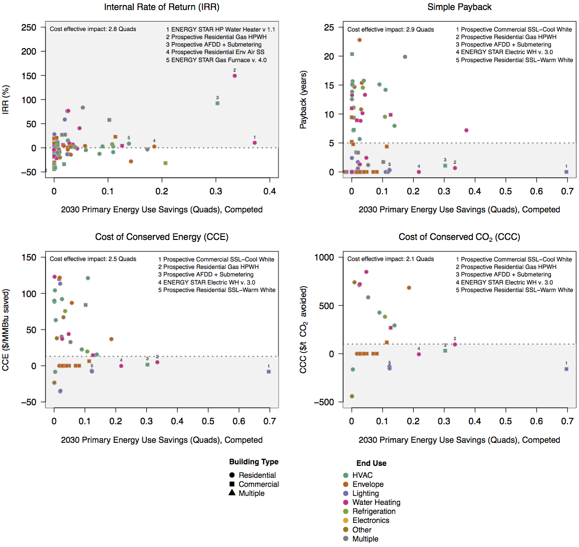
Fig. 6 Each cost-effectiveness figure shows all four cost-effectiveness metrics calculated in Scout for each ECM: internal rate of return, simple payback, cost of conserved energy, and cost of conserved CO2. For this example figure, data from the maximum adoption potential scenario, inclusive of the effects of ECM competition, are shown. Each point corresponds to a single ECM. ECM building type(s) and end use(s) are indicated by each point according to the legend. For the portfolio of ECMs analyzed for this example, the same ECMs generally appear in the list of cost-effective ECMs with the greatest savings, listed in order of total savings in the top right corner of each plot. Solid-state lighting (SSL) ECMs that appear in the other plots are missing from the internal rate of return plot because their calculated incremental installed cost is zero or near zero. Because those technologies have zero/near zero incremental cost, an internal rate of return either cannot be calculated for them or the calculated value is above the plot region’s upper bound. Additionally, several of the ECMs that appear in the internal rate of return and simple payback plots are missing from the cost of conserved energy and CO2 plots; the latter two metrics have a denominator of competed energy savings and avoided CO2 emissions, and these values are zero or near zero for the missing ECMs. Total cost-effective savings, based on the thresholds for each cost-effective metric, indicated by dotted horizontal lines, are generally similar.
Fig. 6 shows an example of the cost-effectiveness figures. All of the cost-effectiveness metrics are plotted against reductions in the metric of interest drawn from a specific year and from one of the two adoption scenarios, 2030 energy savings from the maximum adoption scenario in the case of Fig. 6. The data shown include the effects of ECM competition. The various financial metrics can be used to evaluate the potential cost-effectiveness of the ECMs included in an analysis. The relevance of each metric in evaluating ECM cost-effectiveness will depend on the various economic and non-economic (e.g., policy) factors that might impact the particular individual or organization using these results.
On each plot, a dotted horizontal line represents a target threshold for the given financial metric, and the cost-effective region above or below each threshold is highlighted in gray. The thresholds used are positive IRR, five year payback, the projected U.S. average retail electricity price in the year indicated on the x axis, and the Social Cost of Carbon in the year indicated on the x axis (2.5% average) for IRR, simple payback, CCE, and CCC respectively. Above or below those lines, depending on whether higher or lower values are more favorable for that metric, the ECM might not be cost-effective in its target market. Total cost-effective savings (from all of the ECMs) for the metric of interest shown in the figure are reported in the top left corner of each plot area. Cost-effectiveness thresholds used in the plots should not be considered “official guidance” or canonical, but rather are provided as a starting point for further investigation of the results. Acceptable thresholds for each financial metric vary by building owner and type, thus each threshold shown is an indication of the range around which an ECM might not be cost-effective.
The shape and fill color of each point indicate the applicable building type(s) and end use(s) for each ECM shown on the plot. Comparing the relative locations of these various points might suggest where there are categories that are more generally cost-effective than others. As with the baseline market-aggregated figures, outcomes must be interpreted in light of the particular set of ECMs included in the underlying analysis. In Fig. 6, the top five ECMs pertain to HVAC, water heating, and lighting - each of which constitutes a major end use category with high energy cost savings potential across the residential and commercial building sectors. Generally speaking, ECMs with a high energy performance to cost ratio are most likely to appear in the top five list.
Baseline market-aggregated figures
The results figures with metrics of interest grouped by the baseline market parameters climate zone, building class [12], and end use have file names that begin with the metric of interest, followed by the adoption scenario (coded as “TP” for technical potential or “MAP” for maximum adoption potential), and ending with “-Aggregate,” for example, Total Energy Savings-MAP-Aggregate.pdf.
Each PDF contains three plot areas, one for each of the three baseline market parameters. The x-axis corresponds to the modeling time horizon (by default, years 2015 through 2040), and the y-axis corresponds to the reductions in the metric of interest – energy savings, avoided * |CO2| emissions, or energy cost *savings – indicated in the file name. These plots summarize only the results that account for ECM competition. The dotted line on each plot corresponds to the right side y-axis and represents the cumulative results for all the ECMs in the analysis. The line is the same for all three plots within a single PDF. For these figures, while the data are shown as lines instead of points, the data exist as point values for each year in the modeling time horizon and line segments between each year are interpolated and do not represent actual model data.
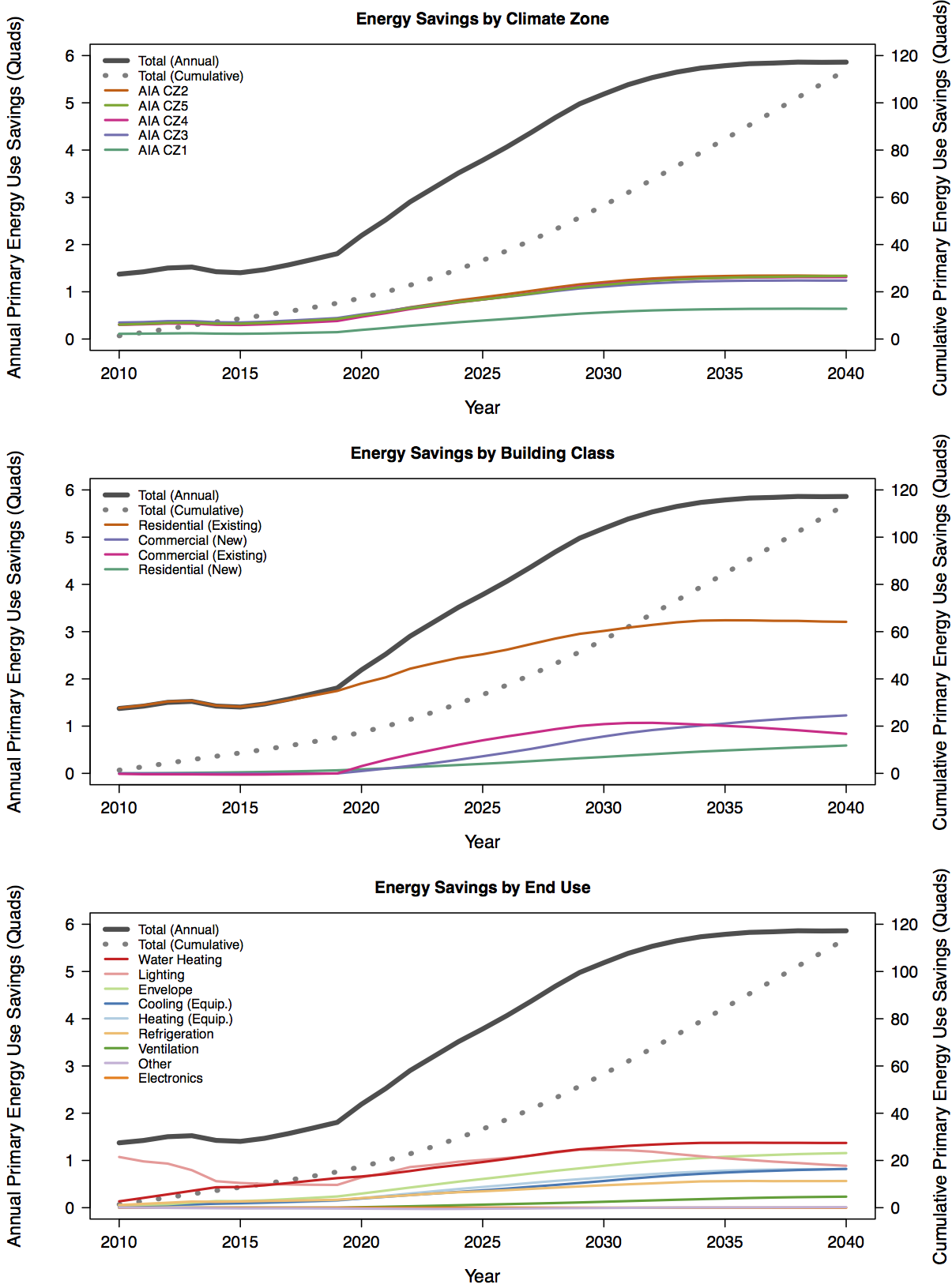
Fig. 7 In this figure, primary energy use reductions are summarized by end use, climate zone, and building class for the maximum adoption potential scenario, including ECM competition. Data are presented for each year in the modeling time horizon (note: this analysis includes ECMs with 2010 market entry years; thus the start year is reset to 2010 from a default of 2015). The majority of total energy savings in 2010 comes from the introduction of a lighting ECM where the baseline lighting technology has a lifetime of less than one year, as can be seen in the end use breakdown plot. As a result of the short baseline lighting lifetime, the entire lighting stock turns over in 2010. After 2010, annual savings for the lighting end use decline through 2015 as baseline lighting efficiency gradually improves and no new lighting ECMs are introduced to the market. Total energy savings are the same for most climate zones except AIA climate zone 1, which has a lower population density and baseline energy use than the other climate zones. The range of results by building class is a result of the comparatively larger baseline energy use reduction potential for existing residential buildings and, before 2020, the poor energy performance of commercial ECMs relative to comparable baseline technologies. Annual energy savings generally increase over time for new buildings, as more new construction accumulates, and reach a ceiling or decline for the existing buildings that are gradually replaced by new construction.
In general, the figures like Fig. 7 can be used to see at a glance the contributions from various end uses to overall results, as well as the distribution of results among building types and climate zones. While some end uses might appear to contribute more to the total annual or cumulative energy savings (or avoided CO2 emissions or cost savings), the baseline energy use is different for each end use, and some end uses might appear to contribute more to the savings in part because their baseline energy use is greater. Similarly, while some building types or climate zones might show greater energy savings (or improvement in other metrics) than others, they may also have significantly different baseline energy use.
These results are highly sensitive to the ECMs that are included in the analysis. While an introductory set of ECMs are provided with Scout, if ECMs added by a user are limited to a single end use, for example, it is reasonable to expect that greater reductions in energy use will come from that end use than other end uses.
In the building class plot, differences in the potential savings from new and existing buildings are a result of the building stock being dominated by existing buildings, thus yielding much larger savings in early years of the modeling time horizon than from new buildings.
For most end uses, ECMs and the baseline technologies have similar lifetimes. As the ECMs in that end use diffuse into the equipment and building stock and comparable baseline technology efficiencies improve, the total savings will gradually reach a ceiling or decline year after year, only yielding further increases if more efficient prospective ECMs become available in subsequent years.
In the version of the Fig. 7 that shows energy savings under the technical potential scenario, there are sharp increases in the energy savings in some end uses. These increases come from several key ECMs that have enough of a disparity in energy efficiency from the baseline technologies to yield dramatic overnight savings. Such increases are a result of the ECM adoption assumptions in the technical potential scenario, and should be viewed as an extreme upper bound on the potential for primary energy use reductions in the end uses, climate zones, and building classes shown.
ECM-specific figures
The figures with results for the metric of interest for each ECM included in the analysis all have file names that begin with the metric of interest, followed by the adoption scenario (coded as “TP” for technical potential or “MAP” for maximum adoption potential), and ending with “-byECM,” for example, Total Cost-MAP-byECM.pdf.
The PDF file includes a single plot for each ECM, with the modeling horizon (by default, years 2015 through 2040) on the x-axis and the parameter indicated in the PDF file name on the y-axis – energy, cost, or CO2 emissions. A legend is included at the end of the figure on the last page of each PDF. Immediately preceding the legend is a summary plot showing the combined effect of all of the ECMs included in the analysis.
The y-axis scale for each plot is adjusted automatically to be appropriate for the data shown. Care should be taken when inspecting two adjacent plots, since what look like similar changes in energy, CO2, or operating cost values at a glance, might in fact be quite different depending on the y-axes. The y-axis markings must be used to determine the magnitudes in the plots and to compare between plots.
Except for the “All ECMs” plot (illustrated in Fig. 8), each plot shows at least four data series. The two darker, thicker lines correspond to the baseline data with and without ECM competition effects (i.e., “competed” and “uncompeted,” respectively) and represent the portion of all U.S. buildings’ energy use (or CO2 emissions or operating cost expenses) that could be affected by the introduction of the ECM shown in that plot. The two thinner, lighter lines correspond to the “efficient” results with and without ECM competition effects and reflect the impact of the introduction of the ECM on the baseline energy, CO2 or operating cost.
These figures are most readily interpreted by comparing relevant pairs of lines.
Uncompeted baseline and competed baseline – the direct or indirect [13] effects of ECM competition on the total baseline market and associated energy, CO2, or cost that can be affected by each ECM
Uncompeted baseline and uncompeted “efficient” – the potential for energy savings, cost savings, and avoided CO2 emissions from the ECM in the absence of alternative technologies that provide the same services
Competed baseline and competed “efficient” – the potential for energy savings, cost savings, and avoided CO2 emissions from the ECM when other ECMs could provide equivalent service but with different energy/CO2/cost tradeoffs
In addition to these comparisons, the uncertainty range (if applicable) around “efficient” results and the effect of that uncertainty on competing ECMs should be examined. Fig. 9 illustrates results for an ECM that includes a probability distribution in its definition and the effect of that distribution on related ECMs.
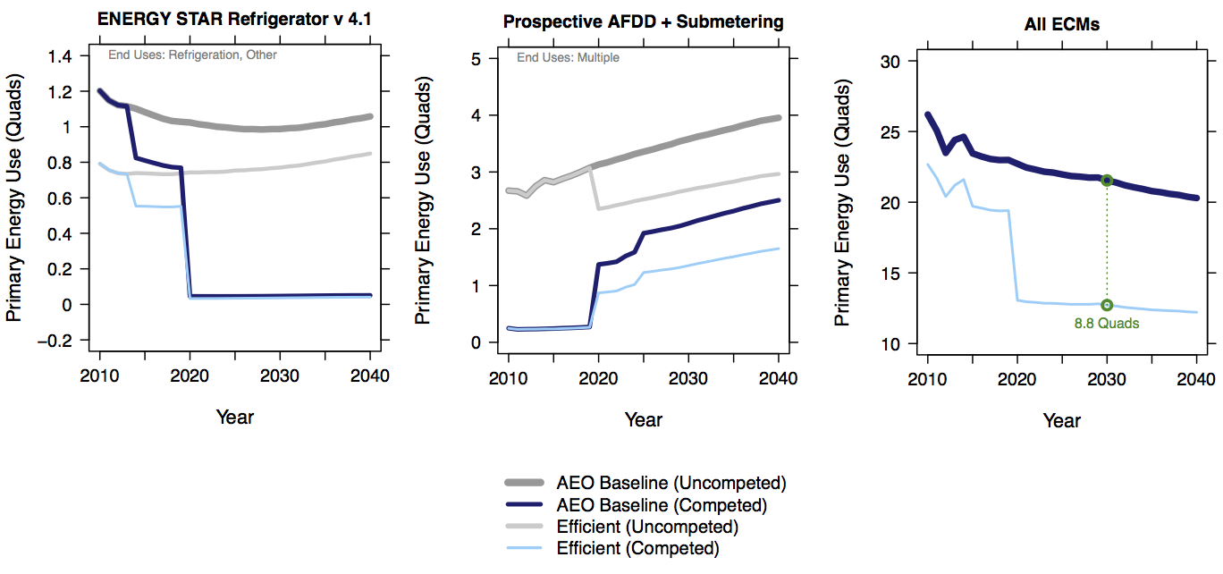
Fig. 8 Primary energy use baselines, and improvements with the adoption of two ECMs – ENERGY STAR Refrigerator v. 4.1 and Prospective AFDD + Submetering – are shown for each year in the modeling time horizon (note: the ENERGY STAR refrigerator ECM has a 2010 market entry year; thus the start year is reset to 2010 from a default of 2015). The data shown are from the technical potential adoption scenario, which is reflected in the abrupt single-year changes in energy use when the ECM enters the market. The data are derived from a model that included many ECMs besides those shown, thus the ECMs’ impacts change under competition. Affected end uses are shown at the top of each plot to help determine which ECMs might be competing with each other. The “All ECMs” figure on the right side shows the aggregate reductions in the metric of interest from all of the ECMs included in the analysis, and the dotted line at the year 2030 indicates the total savings in that year.
When comparing the uncompeted or competed results in plots like those shown in Fig. 8 and Fig. 9, a difference between the baseline (dark) and efficient (light) cases indicates a potential reduction in the metric of interest plotted. In the absence of competition, the efficient case for both ECMs in Fig. 8 show the immediate realization of the entire savings potential upon market entry (2010 and 2020 for the ENERGY STAR refrigerator and Prospective AFDD ECM, respectively), which is characteristic of the technical potential scenario.
While for many categories, the uncompeted baseline will decline into the future as technology improvements and new standards improve the efficiency of the building and equipment stock, there may be cases where the baseline increases over time. In general, this trend arises due to increases in the size of the stock, increases in home square footage (for residential ECMs), or increases in the capacity or size of the equipment (e.g., increases in the interior volume of refrigerators) that outpace improvements in the performance of the applicable equipment or building envelope component. This type of trend in the baseline appears in Fig. 8 for both the ENERGY STAR refrigerator and Prospective AFDD ECMs. Results for some ECMs show large variations in the baseline for years prior to the current year. These variations are an artifact of the configuration of the National Energy Modeling System (NEMS), which is used to generate the AEO projections.
When ECM competition is introduced, the baseline reflects the year of market entry of each ECM and its competitiveness relative to the other ECMs included in the analysis. Prior to the market availability of an ECM, the competed baseline will reflect the portion of the market left over from competing ECMs. Once the ECM is available, it can begin to recapture some of the market, depending on its competitiveness. If the ECM is more competitive, then it will capture a greater portion of the total available market. If the competed baseline appears to follow the same trend as the uncompeted baseline, the ECM is not capturing any (or any more) of the available market. In Fig. 8, the refrigerator ECM captures all of its potential market in its first year of availability, when no competing refrigerator ECMs are on the market; the potential market for this ECM is substantially reduced in 2015, with the introduction of an updated ENERGY STAR refrigerator ECM, and is all but eliminated in 2020, with the introduction of a prospective refrigerator ECM that satisfies aggressive cost and performance targets (competing refrigerator ECMs not shown). Conversely, the potential market for the Prospective AFDD ECM in Fig. 8 grows after its market introduction; this growth continues between 2020-2025, when the introduction of additional ECMs reduces the market share of ECMs that compete with the Prospective AFDD ECM, thus increasing its potential market.
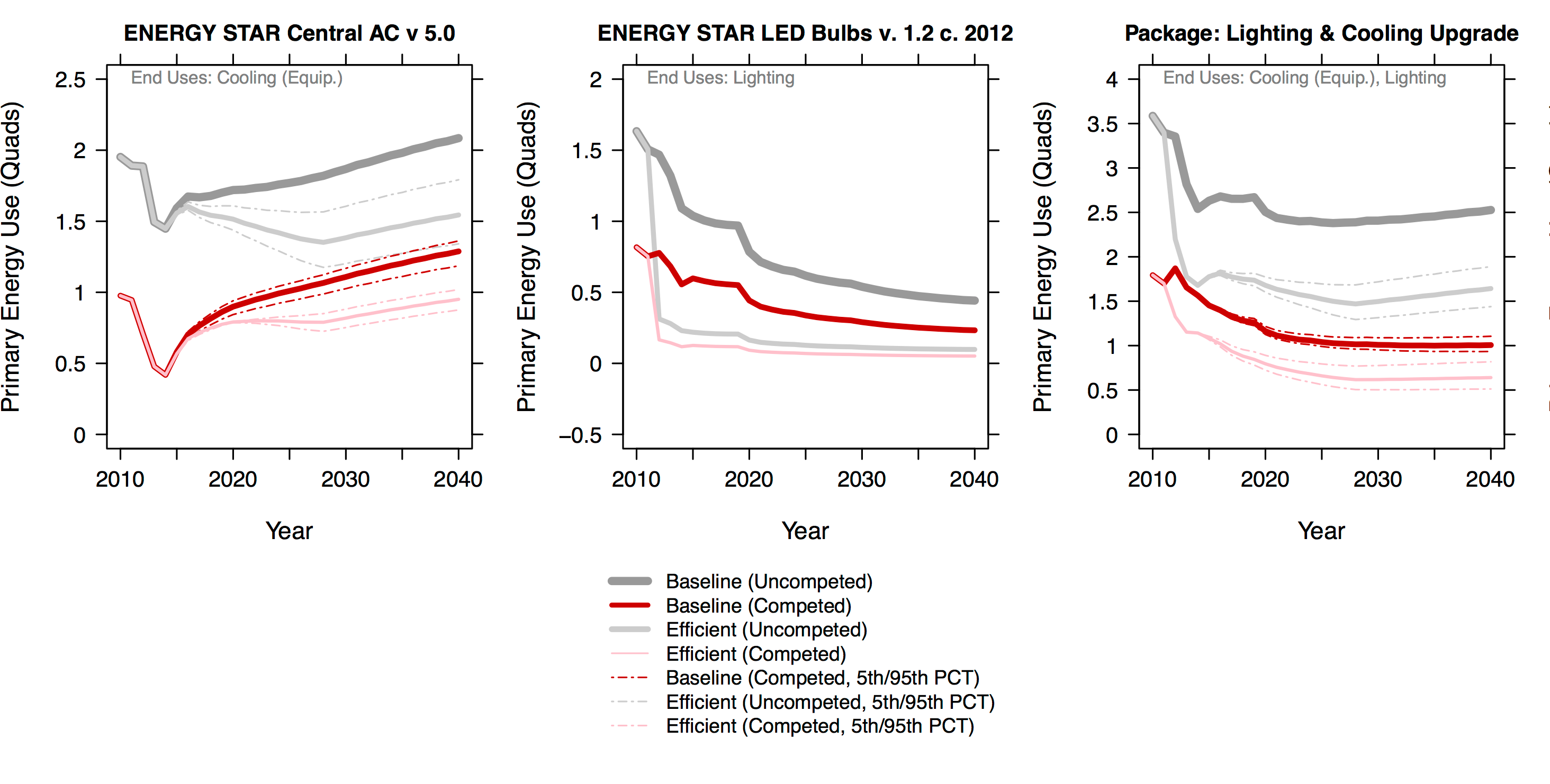
Fig. 9 The ENERGY STAR Central AC ECM includes a probability distribution on one or more of the installed cost, efficiency, or product lifetime, which is reflected in the results. The 5th and 95th percentile bounds for each affected value are shown with dashed lines of the same color. The two ECMs shown on the left are combined into the package ECM on the right. The package ECM results reflect the effect of the probability distributions in the contributing ECMs.
The effect of probability distributions are reflected in the results of the ECMs that include them in their definitions, as well as in the competed results for any competing ECMs and in any packages that include the ECM. The effects of uncertainty will always appear in the results with the ECM applied (i.e., the “efficient” results), though if the spread of the distribution is quite small, it might be difficult to see the dashed lines showing those effects in plots Fig. 9. In addition, if a probability distribution is applied to the installed cost or energy efficiency of the ECM, it will create uncertainty in the capital and/or operating cost of the ECM, and thus will introduce uncertainty in ECM competition, which is reflected in the competed baseline for the ECM. The ENERGY STAR air conditioning ECM in Fig. 9 shows this effect.
Viewing tabular outputs
The plot generation script plots.py also produces Excel-formatted files containing summaries of the results. The summary results for each adoption scenario are stored in the corresponding scenario folder within the ./results/plots directory. The structure of the results in the files corresponding to each scenario is identical. Each file has three tabs, corresponding to energy use, CO2 emissions, and energy cost results. These results correspond to the data that are shown in the ECM-specific plots, as in Fig. 8, and the tabular results can be used to create custom visualizations different from those automatically generated with plots.py.
Tip
If you are experienced with matplotlib, you can also modify plots.py to tailor the figures to your preferences.
On each tab, the first five columns provide information about the ECM and the type of data reported in each row. The first column contains the name of the ECM for the data in each row and the third through fifth columns provide details regarding the climate zones, building classes, and end uses that apply to each ECM. The second column indicates the type of data in each row – one of the four series shown in Fig. 8, the baseline and efficient results, with and without ECM competition. The sixth through ninth columns contain results for the financial metrics: internal rate of return (IRR), simple payback, cost of conserved energy (CCE), and cost of conserved CO2 (CCC). When any of the financial metrics cannot be calculated (e.g., simple payback for a negative incremental capital cost, or negative energy cost savings) the metric will be reported as the value 999. The columns beyond the ninth column contain the results for the metric of interest (energy use, CO2 emissions, or energy cost) indicated by the worksheet tab name. Each of those columns corresponds to a year in the simulation, with the year indicated in the first row.
For a given set of results data on a single tab, each ECM included in the simulation appears in four rows that are distinguished by the ECM’s name (listed under the “ECM Name” column). These four rows correspond to the uncompeted and competed baseline results, as well as the (“efficient”) results with the ECM applied, again with and without competition. For each ECM, these rows correspond to the four primary lines that appear in the ECM-specific results figures, as in Fig. 8.
In each results tab, rows 2-22 include results summed across the entire ECM portfolio (rows with “All ECMs” listed under the “ECM Name” column). The information in these 21 rows is interpreted as follows: rows 2-3 show competed baseline and efficient results summed across the entire ECM portfolio - these rows correspond to the two primary lines that appear in the “All ECMs” plot in the ECM-specific results figures; row 4 shows the difference between the competed baseline and efficient results shown in rows 2-3 (“Baseline - efficient”); and rows 5-22 break down the result shown in row 4 by climate zone (5 climate categories/rows), building type (4 building type categories/rows), and end use (9 end use categories/rows).
Note
For each ECM in the results, in addition to the total energy use, CO2 emissions, and energy cost results contained in the Excel files, the ecm_results.json file includes those results broken out by each of the applicable baseline market parameters – climate_zone, bldg_type, structure_type, fuel_type, end_use, and technology – that apply to each ECM. These results breakdowns are provided for both the baseline and efficient cases (without and with the ECM applied, respectively).
Footnotes